Notebooks

Notebook Examples

This branch contains 38 notebooks. The page inventories every one of them; the output cards below are published separately and are described under Verified notebook outputs.

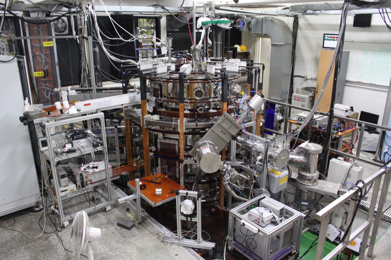
VAFT overview

How to read this index

The notebooks are at two different levels of maturity, and it saves a lot of time to know which is which before you open one:

  • Runnable — the notebook contains executable cells and a working data path. 27 notebooks.
  • Design shell — the notebook is currently a structured markdown outline (objectives, expected inputs and outputs, planned sections) with no code cells yet. 11 notebooks. They are useful as specifications of where a pipeline stage is heading, but they will not execute anything.

Design shells are marked (design shell) below.

Verified notebook outputs

The figures below were exported on 2026-08-21 with MPLBACKEND=Agg and VAFT_DOCS_READ_ONLY=1, from a commit and a branch that no longer exist, by an exporter that has since been removed from the repository. Every image still matches its recorded checksum, but none of them can be tied to the notebook that produced it, because the notebooks have moved on. They are kept as legacy artifacts and are labelled as such in _data/notebook_outputs.yml; regenerating them is tracked in issue #156. Treat them as illustrative, not as current output.

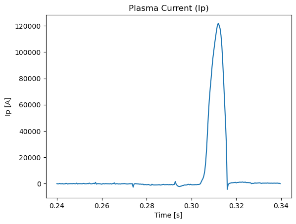
Offline first result

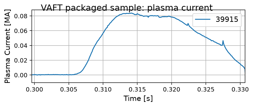
Line plot of VEST shot 39915 plasma current from 300 to 330 milliseconds.
Plasma current from the packaged offline sample.
Execution provenance
Notebook
notebooks/database_initialization_and_load.ipynb
Notebook SHA-256
f7c97ecf5f92a355e870cc0d77b0006cf4fa437f5e49e638db856dd5be53df3f
Execution mode
offline-packaged-data
Data
Packaged OMAS sample for VEST shot 39915
Shot / time
39915 / 0.300–0.330 s
Python / VAFT
3.12.9 / 0.5.0
Executed
2026-08-21T21:40:52+09:00
first-result.png SHA-256
9301167e833591d9591c6463b60269be75f22c0e1e8d47008d9f167216cd828e

Public HSDS shot 39915 metadata

Open TXT artifact — Lazy-ODS metadata returned by a live read-only HSDS request.

Execution provenance
Notebook
notebooks/database_initialization_and_load.ipynb
Notebook SHA-256
f7c97ecf5f92a355e870cc0d77b0006cf4fa437f5e49e638db856dd5be53df3f
Execution mode
read-only-public-hsds
Data
public/39915/equilibrium
Shot / time
39915 / 0.316–0.327 s
Python / VAFT
3.12.9 / 0.5.0
Executed
2026-08-21T21:40:52+09:00
hsds-39915.txt SHA-256
b638972489ba5c784ec52851a624be8d9f6d09706cb91d93b2a9d94cb72f65a6

OMAS and IMAS-path round trip

Open TXT artifact — Root-IDS comparison before and after a local compressed-JSON round trip.

Execution provenance
Notebook
notebooks/read_and_convert_data_structure.ipynb
Notebook SHA-256
ab0bdecbfe70ed117ccac0611f8dcd994d1feaee889645f0236365c3fd5a95bc
Execution mode
offline-temporary-directory
Data
Packaged OMAS sample
Shot / time
39915 / not-applicable
Python / VAFT
3.12.9 / 0.5.0
Executed
2026-08-21T21:40:52+09:00
imas-roundtrip.txt SHA-256
5e0522ddb6c3c459d38c96a5261350b45ca84fa58d61f69c9094609c4f1505b2

Archived-shot Mirnov spectrogram

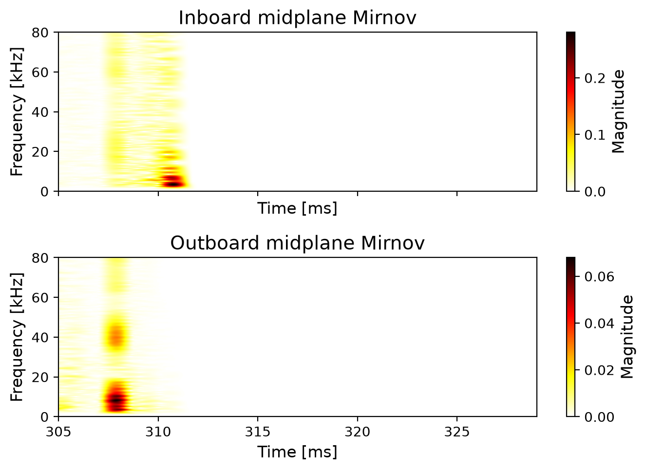
Two stacked spectrograms showing Mirnov fluctuation magnitude up to 80 kilohertz.
Inboard and outboard Mirnov power spectra from archived shot 44740.
Execution provenance
Notebook
notebooks/fluctuation_diagnostics_analysis.ipynb
Notebook SHA-256
a41968189104e0047c9867e1e0b772ca2f1519da270bd384cdf1fd89ea11e21a
Execution mode
offline-archived-shot
Data
vaft/data/legacy/shot_44740.json.gz
Shot / time
44740 / 0.304–0.330 s
Python / VAFT
3.12.9 / 0.5.0
Executed
2026-08-21T21:40:52+09:00
mirnov-spectrogram.png SHA-256
17c631ea70e35f0383f66c53b6adec638df27f7cedee9edd4c302fb22ec899f1

Paired kinetic-profile result

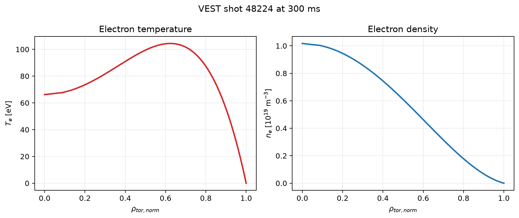
Side-by-side electron temperature and density profiles for VEST shot 48224 at 300 milliseconds.
Electron temperature and density profiles generated on a 129-point normalized-flux grid.
Execution provenance
Notebook
notebooks/kinetic_efit_end_to_end.ipynb
Notebook SHA-256
789fdf1591de3f8d87777e9bcb6f8c549a6f43f0bcf535900735782c2f3915f2
Execution mode
offline-paired-diagnostics
Data
Repository GEQDSK, Thomson and ion-Doppler files
Shot / time
48224 / 0.300 s
Python / VAFT
3.12.9 / 0.5.0
Executed
2026-08-21T21:40:52+09:00
kinetic-profile.png SHA-256
a90e3861a2c18382e478a24526b8a5354d769266e679744d56362215028a7453

Equilibrium input preparation

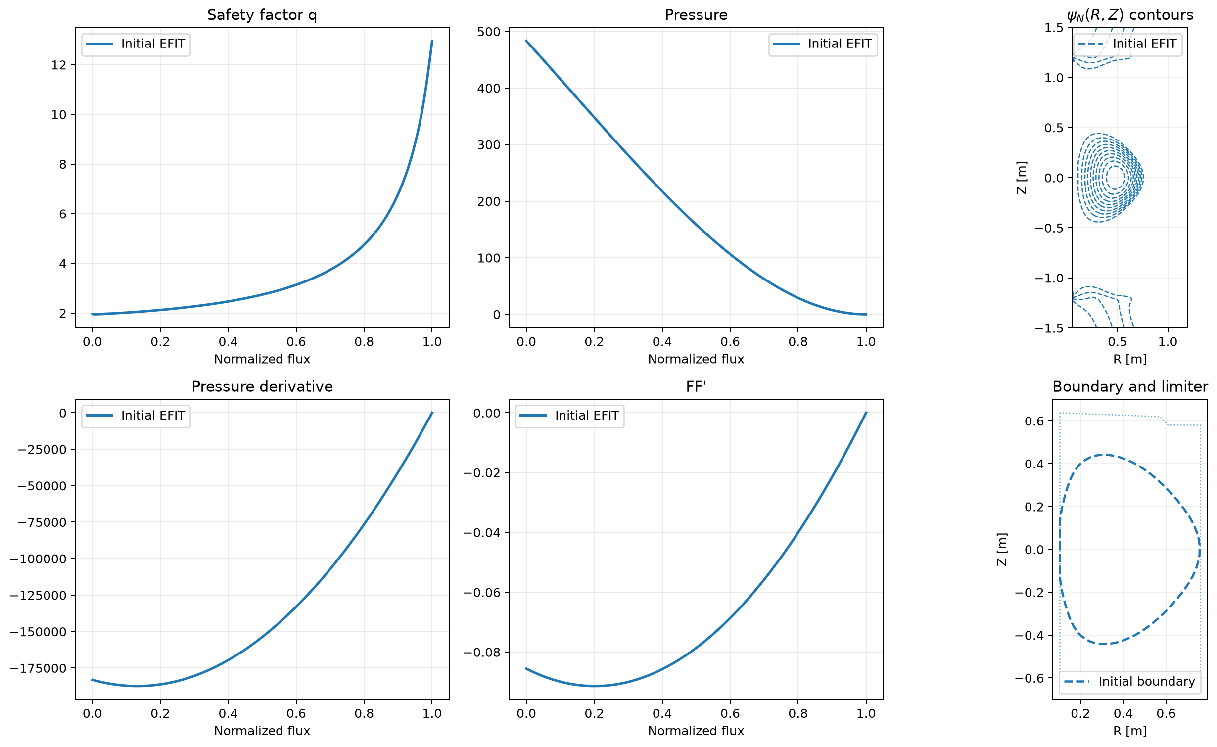
Six-panel equilibrium input figure with profiles, normalized-flux contours, boundary and limiter.
EFIT profiles, flux contours and boundary used to prepare CHEASE inputs.

Open TXT artifact — Prepared-file and executable-readiness report.

Execution provenance
Notebook
notebooks/equilibrium_refinement_using_chease.ipynb
Notebook SHA-256
9e2b221eab484bbba055e0aed1a9690c831233c4f4a7df2bf5fc05f26ff0de8c
Execution mode
deterministic-input-preparation
Data
vaft/data/efit/g039915.00319
Shot / time
39915 / 0.319 s
Python / VAFT
3.12.9 / 0.5.0
Executed
2026-08-21T21:40:52+09:00
equilibrium-inputs.png SHA-256
680abc32c64b5e9ba8b296cec3468e1e128a9fef2d35b3c9de094fa4ed28e0c7
equilibrium-readiness.txt SHA-256
14b3d14bb3ab6776adb80e7e4078499a9211d4bff0f3de9907055e112882f3bc

External-code readiness

Open TXT artifact — Optional external-code configuration status without credential or secret values.

Execution provenance
Notebook
notebooks/initialize_external_fusion_codes.ipynb
Notebook SHA-256
a7169d5ceb351ee781d059ba8189e46b7ab696e67a39723484cac25d29ebbdaf
Execution mode
read-only-environment-inspection
Data
GPECHOME, CHEASEHOME, EFITHOME and TESHOME
Shot / time
not-applicable / not-applicable
Python / VAFT
3.12.9 / 0.5.0
Executed
2026-08-21T21:40:52+09:00
external-code-readiness.txt SHA-256
5412b49b5173c00f81d994d25e585d0b2e0c28cfef8df5cb1ccbb34b7b665708

Confinement-scaling result

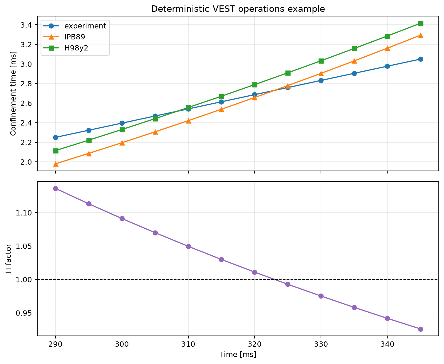
Two-panel plot comparing confinement-time estimates and the IPB89 H factor.
Experimental and empirical confinement times with the IPB89 H factor.

Open TXT artifact — Row count and mean confinement metrics.

Execution provenance
Notebook
notebooks/confinement_time_scaling.ipynb
Notebook SHA-256
02f602010db261dd6eb71cbba5334ad2854e325c14907bfb325c56d85979f812
Execution mode
deterministic-offline-analysis
Data
Pinned synthetic operations-analysis fixture
Shot / time
not-applicable / 0.290–0.345 s
Python / VAFT
3.12.9 / 0.5.0
Executed
2026-08-21T21:40:52+09:00
confinement-scaling.png SHA-256
d589ce0aa5c2a8669532a7832f1a7464854d204da5b11d479bef4bd81ebb705d
confinement-scaling.txt SHA-256
0e0a93ed6eb137150fe0a0991db52306bd14fb5caffd8386789bd02c2d04c393

Snakemake pipeline stage summary

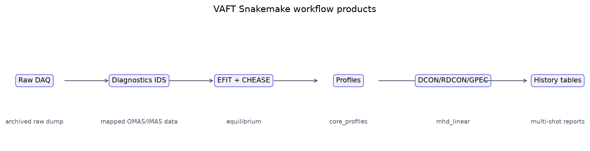
Horizontal diagram from raw DAQ through diagnostics, equilibrium, profiles and MHD products to history tables.
Routine, corrective and summary products in the VAFT Snakemake workflow.

Open TXT artifact — Machine-readable workflow stage and output summary.

Execution provenance
Notebook
notebooks/automated_pipeline_overview.ipynb
Notebook SHA-256
a04dd9ff3b1c8b9a6a4b888374977a041b1236e7644a1d8ae71d99904657250f
Execution mode
deterministic-offline-diagram
Data
Pinned workflow-stage definition
Shot / time
not-applicable / not-applicable
Python / VAFT
3.12.9 / 0.5.0
Executed
2026-08-21T21:40:52+09:00
pipeline-overview.png SHA-256
8c78973028a647a5a398cfb816ebdc9c040ee621d5f8ff04921550eeee778165
pipeline-overview.txt SHA-256
193e1ba7806cc3ebb3d41f53391264780a48cf0197d03cd55c9bb2e3a83b06ad

Getting started and the database

Notebook Purpose
database_initialization_and_load.ipynb Install VAFT, verify the HSDS connection, list public shots, and load a shot into an ODS.
vest_experimental_data_list.ipynb Tour of IMAS/OMAS concepts and of which VEST diagnostics are mapped into the database today.
vest_raw_signal_sql_database.ipynb Reach the legacy SQL DAQ store: field codes, slow vs fast channels, and raw waveform retrieval.
verify_exist_shot_and_load.ipynb Inspect published-shot status and verify selected read paths without changing the remote namespace.

Start here. This is the shortest path from a fresh install to a shot in memory.

import vaft

# Is the HSDS backend reachable?
print(vaft.database.is_connect())

# Which shots are published?
shots = vaft.database.exist_shot("public")

# Load one shot as an OMAS ODS
ods = vaft.database.load(39915, source="public")

vaft.database.load is the canonical entry point: it returns an OMAS ODS, and it also accepts an explicit ids_name= keyword when you want a native IMAS IDS instead. See Database for the full surface.

If you have no network access, every example below can also be driven from the packaged sample data described in the next section.

Data structures and IMAS

Notebook Purpose
read_and_convert_data_structure.ipynb Walk an equilibrium ODS key by key — equilibrium.time_slice, profiles_1d, and the rest of the hierarchy.
imas_omas_data_conversion.ipynb Bridge OMAS ODS objects and native IMAS AL5 HDF5 storage, in both directions.

The packaged samples are the fastest way to get a realistic ODS without touching the network:

import vaft

ods = vaft.omas.sample_ods()   # one shot

list(ods.keys())
print(ods["equilibrium.time"])
print(list(ods["equilibrium.time_slice.0"].keys()))

To reach another registered shot, or the same shot in a different representation, ask the sample registry:

import vaft

vaft.data.available_samples()                          # (39915, 41524, 41672)
sample_path = vaft.data.sample(39915)                  # packaged OMAS artifact
imas_path = vaft.data.sample(39915, representation="imas")   # repository checkout only

A pip install vaft carries only the OMAS form of 39915 (omas.json.gz, which both adapters read); its IMAS netCDF twin imas.nc is repository-only, so representation="imas" raises a FileNotFoundError naming the file from an installed wheel and needs a Git checkout.

For the IMAS round trip:

import tempfile

entry_dir = tempfile.mkdtemp(prefix="vest_imas_")
vaft.imas.save(ods, entry_dir)
ods_back = vaft.omas.load(entry_dir)

Related reading: Data structures and Machine mapping.

Diagnostics

Notebook Purpose
magnetic_diagnostics_processing.ipynb (design shell) Planned preprocessing, filtering, calibration, and sign conventions for ip, flux loops, and poloidal probes.
soft_x_ray_signal_analysis.ipynb Map digitizer CSVs into a soft X-ray ODS, then plot lines of sight, signals, and spectrograms.
analytic_island_model_and_synthetic_response_model.ipynb Put an analytic m/n magnetic island on an equilibrium (Solov’ev and its CHEASE refinement) and compute the synthetic VEST soft X-ray chord response as it rotates.
fluctuation_diagnostics_analysis.ipynb Mirnov coil fluctuation work: spectrograms, toroidal mode spectra, and mode-number fits.
fast_camera_video_analysis.ipynb (design shell) Planned camera image and video loading, plasma-behavior observation, and synchronization.

Probe example

The soft X-ray notebook is a good template for “raw file to ODS to plot” in one pass:

import vaft
from vaft.machine_mapping.soft_x_rays import soft_x_rays_from_digitizer_csv

ods = soft_x_rays_from_digitizer_csv(shot, daq_label, digitizer_file=plasma_file)

vaft.omas.plot_soft_x_rays_geometry_lines_of_sight(ods, selection=["lowermid", "bottom"])
vaft.omas.plot_soft_x_rays_time_power(ods)
vaft.omas.plot_soft_x_rays_spectrogram(ods)

See Magnetics and Processing.

Equilibrium and stability

Notebook Purpose
equilibrium_refinement_using_chease.ipynb Refine an EFIT g-file with CHEASE and qualify the result: the boundary and profiles CHEASE is given, the q95 constraint, sign conventions, what the solve changes, solver-mesh convergence, and target_psin/relax sensitivity.
fixed_boundary_parametric_scan_using_chease.ipynb Local fixed-boundary sensitivity of a CHEASE equilibrium: pressure, current-peaking and shape scans kept apart as requested, materialized and achieved, a pressure x peaking grid, a response matrix, and failed cases kept as results.
generate_0d_synthetic_equilibrium_using_chease.ipynb A fixed-boundary CHEASE equilibrium from 0D descriptors and explicit source shapes: current or q95 normalization, requested vs achieved, and why one 0D description has many equilibria.
forward_equilibrium_using_TES.ipynb Forward (Grad-Shafranov) equilibrium solve with TES, driven straight from an ODS.
forward_equilibrium_using_TokaMaker.ipynb Forward free-boundary equilibrium with TokaMaker (Open FUSION Toolkit), driven by measured PF coil currents.
time_dependent_equilibrium_using_TokaMaker.ipynb Vessel eddy currents, wall eigenmodes, quasi-static shot evolution, and vertical-stability growth rates with TokaMaker.
free_boundary_pf_coil_scan.ipynb Free-boundary PF-coil-current scans: commanded against materialized currents, per-case topology classification, and resumable continuation.
conference_operational_space_atlas.ipynb The #1331 Tier A good and admissible EFIT states on literature operational-space projections (β_N–l_i, Troyon, q95–l_i, Wesson l_i–q_ψ), coloured by the kinetic, stability and transport atlas layers. Needs the atlas tables in $VAFT_ATLAS_DIR (vestserver campaign outputs).
stability_atlas_population.ipynb The Tier A stability atlas population: DCON ideal W_t (n = 1–6), RDCON/STRIDE Δ′_max (n = 1, 2) and the Mercier/ballooning criteria as three histograms against their stability boundaries. Needs the atlas tables in $VAFT_ATLAS_DIR (vestserver campaign outputs).
analytic_solovev_equilibrium.ipynb Constant-source analytic Solov’ev construction, verified against the gridded field; a VEST-like analytic baseline with Miller characterization, descriptors and geometry/source scans.
analytic_guazzotto_freidberg_equilibrium.ipynb Guazzotto–Freidberg analytic equilibria with vanishing edge pressure and current: the paper’s Table 4 reproduced, a VEST-like shape in three topologies, and the contrast with Solov’ev.
analytic_fixed_to_free_boundary.ipynb Execute 20 analytic fixed-to-free cases with independent direct Green and TokaMaker get_vfixed() fits, then compare initial, refined and final current-frozen results. The notebook stores compact tables and figures; fresh native solves require an installed OFT.
analytic_plasma_state_presets.ipynb Synthetic L-mode, H-mode, ITB and H-mode + ITB kinetic states on one fixed Solov’ev geometry: derived pressure and gradients, barrier semantics, the projection onto (R, Z), and why a prescribed state is not a self-consistent equilibrium.
synthetic_kinetic_profiles_from_equilibrium.ipynb Synthetic kinetic profiles from a real and an analytic equilibrium, fidelity Levels 0-3: equilibrium-constrained against kinetic pressure closure with residuals, composition and Z_eff, the core_profiles output, and what is assumed rather than derived.
self_consistent_equilibrium_kinetic_iteration.ipynb An assumption-driven self-consistent equilibrium and kinetic-profile state: the equilibrium pressure decomposed, or CHEASE re-solved for the kinetic pressure until the two agree, with the iteration history, the current policy, what is held and what is recomputed, and the failure states.
compact_equilibrium_representation.ipynb Compact representations of an existing equilibrium with their fidelity: the best Solov’ev fit and the MXH-Chebyshev representation of Xie and Li, and how its error falls with the number of parameters.
equilibrium_representation_reference.ipynb One EFIT equilibrium through every representation VAFT has: four radial coordinates, flux map, PEST grid, Miller and Fourier fits, kinetic profiles and a/L_T, rational surfaces, a prescribed island, a 3-D embedding and a camera projection, with the same source, time, COCOS and flux unit checked at each step and the gaps named.
local_miller_equilibrium_fitting.ipynb Local Miller fitting, its reconstruction errors, and where it stops working near the separatrix.
parametric_equilibrium_descriptors.ipynb Convention-aware global descriptors, and GEQDSK against ODS parity.
edge_and_boundary_representation.ipynb Limiter and diverted topology, X-points, gaps, and separatrix balance.
initialize_external_fusion_codes.ipynb Read-only readiness checks for the GPECHOME, CHEASEHOME, EFITHOME, and TESHOME conventions.
electromagnetic_response_modeling_with_efund.ipynb (design shell) Planned EFUND response modeling over wall geometry, PF active and PF passive structures.
eddy_current_calculation_and_startup_analysis.ipynb (design shell) Planned PF-passive eddy-current ODE solve and tokamak startup / null analysis.
magnetic_equilibrium_reconstruction_with_efit.ipynb (design shell) Planned EFIT reconstruction from magnetics, eddy currents, and PF coil information.
convergence_study_of_efit.ipynb EFIT’s Picard trajectory per slice (#1038): chi-square, flux increment and magnetic-axis height at every iteration, and NXITER=1 against NXITER=3, read from saved iteration histories without running EFIT.
mhd_equilibrium_analysis.ipynb (design shell) Planned equilibrium loading, representative quantities, and coordinate transformations.
linear_ideal_stability_analysis_with_dcon.ipynb Ideal MHD stability (delta-W by toroidal mode) with DCON, run on the packaged VEST equilibrium and mapped into mhd_linear. Needs $GPECHOME.
linear_resistive_stability_analysis_with_rdcon.ipynb Resistive stability with RDCON: the classical tearing index per rational surface, mapped into ntms.deltaw. Needs $GPECHOME.
perturbed_equilibrium_and_3d_response_with_gpec.ipynb (design shell, two sections implemented) Planned perturbed equilibrium and non-axisymmetric 3D response with GPEC. The resonant-response section (#1884) optimizes coil phasing against a GPEC-verified operator Φ = H·conj(c), with core and edge windows from the fitted pedestal; every optimum is confirmed by a direct GPEC run. The NTV torque section (#1887) replays a committed GPEC → PENTRC scan offline: it qualifies T = cᴴQc at converged PENTRC tolerances, and confirms the optimal coil phasing by direct runs.
vest_nbi_analysis_with_nubeam.ipynb Neutral-beam deposition, heating, current drive and loss accounting for VEST with NUBEAM. Runs the repository’s stored case into a temporary directory; needs $NUBEAMHOME.
neoclassical_transport_with_neo.ipynb Neoclassical transport and bootstrap current for VEST with NEO (GACODE). Converts the packaged 48224 kinetic state to input.gacode, runs NEO into a temporary directory, maps the result into IMAS, and compares it with the Sauter and Redl analytic models; needs $GACODEHOME and $GACODE_PLATFORM, and without them each section reports what it would show and the analytic comparison still runs.
turbulent_transport_with_tglf.ipynb Turbulent transport for VEST with TGLF (GACODE) and the TGLF-NN surrogate. Builds the local TGLF input at five surfaces from the packaged 48224 kinetic state, runs TGLF, and audits every public TGLF-NN family against the same input – none is in domain, because VEST’s ion-to-electron temperature ratio is an order of magnitude below every training set. Needs $GACODEHOME and $GACODE_PLATFORM for the native run and $TURBULENTTRANSPORTHOME for the models; the audit needs neither GACODE nor onnxruntime, and without any of them the temperature-ratio finding still runs.

CHEASE is the most complete code-coupling example in the repository. The prepare_* / run_* / collect_* triple is the pattern every code wrapper in vaft.code follows:

from vaft.data import read_geqdsk
from vaft.data.resources import data_path
from vaft.code.chease import CHEASEConfig, prepare_chease_inputs, find_chease_executable

initial = read_geqdsk(data_path("efit/g039915.00319"))
ods = initial.to_omas()

config = CHEASEConfig(workdir=workdir)
inputs = prepare_chease_inputs(initial, config)   # writes EXPEQ + chease_namelist

executable = find_chease_executable(config)       # None if CHEASE is not installed

TES shows the same idea starting from a database shot rather than a file:

import vaft
from vaft.code import tes

ods = vaft.database.load(39915)

cfg = tes.TESConfig(
    executable=RTES,
    workdir=WORKDIR,
    shot=39915,
    time=0.325,
    bt0=0.15,     # fix the toroidal field; omit to read it from the tf IDS
    eddy=True,    # treat pf_passive as eddy coils
)
inputs = tes.prepare_tes_inputs(ods, cfg)

Both binaries are optional: the notebooks degrade to input generation when the executable is absent. See Equilibrium and Stability.

Profiles and transport

Notebook Purpose
profile_fitting_using_equilibrium_and_kinetic_diagnostics.ipynb Map Thomson scattering onto equilibrium flux surfaces to fit core Te and ne profiles.
kinetic_efit_end_to_end.ipynb Build electron and ion profiles from the paired shot 48224 repository inputs at 300 ms.
confinement_time_scaling.ipynb Single-shot workflow test, then a dataset-wide confinement-time scaling and regression study.
single_machine_confinement_scaling_and_dimensional_analysis.ipynb What a single machine can identify: engineering-fit diagnostics, exact Buckingham-Pi groups, the Connor–Kadomtsev constraint from its assumption, and the engineering/dimensionless equivalence test (#1621).
vest_ordering_and_model_applicability.ipynb Which asymptotic orderings, and so which reduced models, the VEST Tier A population supports: ordering margins, the 15 #1627 contracts, radial and temporal applicability, and representative states for downstream studies (#1629).
tokamak_power_balance.ipynb Ohmic input against radiated and conducted losses, with an Aurora-based impurity treatment.
self_consistent_kinetic_inference_vest_39915.ipynb Matched kinetic state for VEST 39915 at 316 ms from an archived, hash-pinned case: a magnetic pressure-partition branch with inferred T_i, and an electron-kinetic EFIT that is rejected for negative edge pressure. Pressure, density, temperature and plasma Z_eff profiles render offline in 2×2 and 4×1 layouts.
self_consistent_kinetic_inference_vest_40326.ipynb Matched kinetic state for VEST 40326 at 322 ms from an archived case: pressure-partition T_i from the magnetic equilibrium next to an admissible electron-kinetic EFIT, with the equal C/O composition assumption and the circular-T_i refusal made explicit.

The profile notebook is the largest runnable example that stays inside pure VAFT:

import vaft

ods = vaft.database.load(40330, source="public")

vaft.omas.plot_thomson_scattering_geometry_poloidal(ods)
vaft.omas.plot_thomson_scattering_time_electron_temperature(ods)
vaft.omas.plot_electron_temperature_profile(ods)

See Profiles and Formula.

Analysis, V&V, and publication

Notebook Purpose
plotting_sample_using_vaft_plot_module.ipynb The plot module tour: naming conventions, ODS vs ODC input, and time-convention shifts.
publication_figures.ipynb Reproduce publication-quality composite figures at print DPI.
verification_and_validation.ipynb Tier A Atlas V&V, offline from a dated snapshot: Thomson against EFIT pressure (channel sums, TS-covered and full-plasma volume ratios), E1/E2/E3 virial identity residuals, volume vs pair-13 beta_p and l_i, and EFIT constraint quality by cohort, on the #1835 population contract (vaft.validation.kinetic_population). VAFT_ATLAS_DIR selects a newer Atlas.
multiple_tokamak_comparison.ipynb (design shell) Planned cross-device comparison of geometry, equilibrium, and diagnostic signals.
multi_machine_confinement_database.ipynb Published multi-machine databases in common VAFT semantics (#1205): ITPA DB5.2.3 confinement and VEST in one confinement table, TCV and ITPA TC-26 L-H transitions in one event table, ITPA PR08 profiles mapped to ODS and overlaid on VEST, with IMAS mapping coverage and source definitions. Needs network; TC-26 from a local copy.
multi_machine_operation_space_database.ipynb Public equilibria from seven machines on every registered operational-space projection the equilibrium alone supplies (#1620): one COCOS-11 state table, projections found from the registry, registered boundaries with their basis and calibration machines, ST and conventional populations kept apart; the VEST Tier A atlas joins through vaft.omas.atlas_state_table when $VAFT_ATLAS_DIR is set. Needs network.

Canonical plots are named vaft.omas.plot_{subject}_{view}[_{quantity}] — the subject is the physical thing, not the IDS that stores it, so the plasma current is plot_plasma_current_time. Any adapter accepts a single ODS, an ODC, or a list of ODS objects, which is what makes shot overlays trivial:

import vaft
from omas import ODC

ods = vaft.omas.sample_ods()

odc = ODC()
for key, shot in enumerate(vaft.data.available_samples()):
    odc[key] = vaft.omas.load(vaft.data.sample(shot))

vaft.omas.plot_plasma_current_time(ods)
vaft.omas.plot_plasma_current_time(odc)   # overlays every shot in the collection

# Re-zero the time axis on breakdown, then replot
vaft.omas.change_time_convention(ods, convention="breakdown")
vaft.omas.plot_plasma_current_time(ods)

Magnetics example

Composite figures are single calls — here the vacuum flux map drawn over the machine geometry:

import vaft

ods = vaft.omas.sample_ods()
vaft.omas.plot_equilibrium_field_psi_vacuum(ods, overlay=("coils", "wall"))

vaft.omas.available_plots() prints the full catalogue, and available_plots(ods) narrows it to what one input can actually draw.

Operations and monitoring

Notebook Purpose
vest_daily_monitoring.ipynb Day-to-day shot health check: load the day’s shots into an ODC and compare key signals.
shot_characteristics_classification.ipynb (design shell) Planned representative-signal extraction, shot classification, and summary sheets.
automated_pipeline_overview.ipynb Deterministic stage and product summary for routine, corrective, and history-table Snakemake paths.

These pair with the automated Snakemake stages described in Pipelines.

Notebook maturity and remaining legacy APIs

The nine documentation-allowlisted notebooks are repaired on the companion branch. Some other runnable notebooks retained from the develop baseline still demonstrate older discovery or file-loading APIs; the working forms below are the migration path.

1. vaft.database.exist_ts_file() does not exist. It is called by tokamak_power_balance.ipynb to discover processed shots. There is no replacement helper in the package; supply the shot list directly, as profile_fitting_using_equilibrium_and_kinetic_diagnostics.ipynb now does:

import pandas as pd

core_profile_shots = [40330]
df = pd.DataFrame({"Shot Number": core_profile_shots, "Status": ["core_profile"]})

2. The packaged data moved. Sample files are no longer flat under vaft/data/, and the interim vaft/data/omas/ layout is gone too: each registered shot now lives in vaft/data/samples/{shot}/ behind vaft.data.sample(). Notebooks that still build a path like os.path.join(os.path.dirname(vaft.__file__), "data", "39915.json") will fail. Use the sample helpers or the registry instead:

import vaft

ods = vaft.omas.sample_ods()          # preferred
sample_path = vaft.data.sample(39915) # or resolve the artifact explicitly

A newcomer should work through the runnable notebooks in this order:

  1. database_initialization_and_load.ipynb — install, connect, load your first shot.
  2. read_and_convert_data_structure.ipynb — learn the ODS hierarchy before you plot anything.
  3. plotting_sample_using_vaft_plot_module.ipynb — the plot naming convention pays for itself immediately.
  4. vest_experimental_data_list.ipynb — find out which diagnostics are actually mapped.
  5. profile_fitting_using_equilibrium_and_kinetic_diagnostics.ipynb — the first real physics workflow.
  6. equilibrium_refinement_using_chease.ipynb — how VAFT wraps an external code.
  7. confinement_time_scaling.ipynb — scale up from one shot to the whole dataset.

Then branch by interest: imas_omas_data_conversion.ipynb for interoperability, soft_x_ray_signal_analysis.ipynb and fluctuation_diagnostics_analysis.ipynb for diagnostics, forward_equilibrium_using_TES.ipynb for forward modeling, and publication_figures.ipynb when it is time to write the paper.

If you have not installed VAFT yet, start at Installation and the Quick start guide. The complete function list is in the API reference.

Scientific ML

  • scientific_ml_lifecycle.ipynb: Offline CPU training, grouped evaluation, computational graphs and experiment identity. See the research ML guide for structured sources and GPU qualification.

results matching ""

    No results matching ""