VAFT API
This page is the map of the vaft package: what each subpackage is for, the entry points you are
expected to call, and where the detailed guide for each area lives. The signatures shown here are the
real ones — copy them. How vaft.formula, vaft.process and vaft.code divide the computation, and
when an optional Actor contract would group their realizations, is set out on
Computational layers.
The complete list of what each subpackage publishes – every object in a module’s __all__, with its
signature, summary, deprecation status and source – is generated from the code on every publish:
follow the API link of a subpackage in the table below. docs/api_inventory.yml groups the
modules into those pages and lists the modules that publish nothing yet.
import vaft

vaft.__version__          # '0.5.0' on the inspected develop baseline
Importing vaft is cheap. The top-level package exposes its subpackages lazily (__getattr__),
so import vaft does not drag in omas, imas or matplotlib until you actually touch
vaft.omas, vaft.imas or vaft.plot. A compatibility shim is applied at import time —
vaft.apply_runtime_compat_patches() — which restores NumPy/SciPy APIs that recent releases removed
(trapz, cumtrapz, interp2d) so that OMFIT-derived code keeps working. You never need to call them yourself.
Package map
flowchart TD
    RAW["VEST raw DAQ / SQL"] --> MM["vaft.machine_mapping<br/>raw signals to IMAS IDSs"]
    MM --> DB[("vaft.database<br/>load / save")]
    DB --> ODS["ODS / IDS<br/>(IMAS data model)"]
    ODS --> OMASL["vaft.omas<br/>ODS-aware find_ / compute_ / update_"]
    OMASL --> PROC["vaft.process<br/>signal and EM math"]
    OMASL --> FORM["vaft.formula<br/>closed-form physics"]
    ODS --> PLOT["vaft.plot<br/>figures"]
    ODS --> CODE["vaft.code<br/>EFIT / CHEASE / GPEC / TES / NUBEAM"]
    CODE --> ODS
    ODS --> DATA["vaft.data<br/>GEQDSK I/O"]
    ODS --> IMASP["vaft.imas<br/>OMAS to IMAS Access Layer"]
| Subpackage | Purpose | Deep dive | Generated reference |
|---|---|---|---|
vaft.database |
Load/save VEST shots (ODS, native IDS) and reach the raw SQL DAQ archive | Data structures | API |
vaft.omas |
The ODS-aware API: find_*, compute_*, update_*, sample data |
this page | API |
vaft.process |
Array-in / array-out signal processing, EM response, magnetics chains | Signal processing and EM modeling | API |
vaft.formula |
Pure physics functions: equilibrium, stability, Green’s functions, constants | Formula reference | API |
vaft.machine_mapping |
Raw VEST DAQ to IMAS IDS mapping, plus uncertainty defaults | this page | API |
vaft.plot |
Matplotlib figures straight from an ODS/ODC | this page | API |
vaft.diagram |
Explanatory schematics (magnetic-island topology, …) drawn from vaft.formula and rendered to SVG |
Scientific diagrams | API |
vaft.code |
Adapters for external codes (EFIT, CHEASE, GPEC, TES, NUBEAM, TRANSP) | this page | API |
vaft.data |
GEQDSK read/write, packaged sample files, and atomic and spectral-line identity (vaft.data.atomic, vaft.data.spectroscopy) |
this page | API |
vaft.imas |
OMAS to IMAS Access Layer bridge | Data structures | API |
vaft.validation |
Scientific assessment: benchmarks, comparisons, regression evidence | API | |
vaft.cli |
Command-line workflows over the library APIs | API | |
vaft.mcp |
Local, read-only MCP server over the discovery APIs, for agent clients (vaft[mcp]) |
MCP server | API |
vaft.gui |
Browser GUI over the plot catalog and interactive controls | Browser GUI | API |
vaft, vaft.compat, vaft.ods_access, vaft.spectroscopy (deprecated alias of vaft.data.atomic/vaft.data.spectroscopy, removed in 0.10.0) |
Top level and small utilities | API |
Atomic and spectroscopic concerns follow the same layering as the rest of the package (#1711).
Identity is data: vaft.data.atomic owns elements, isotopes, charge states and species notation
(AtomicSpecies, parse_species), and vaft.data.spectroscopy owns spectral-line identity and the
IMAS processed_line.label codec (SpectralLineIdentity, parse_line_label, parse_emission_term).
Atomic equations are vaft.formula.atomic, and ODS-aware radiation and composition processing is
vaft.process.atomic / vaft.process.impurity. The labels a diagnostic writes belong to
vaft.machine_mapping, and selecting and presenting lines belongs to vaft.plot. An AtomicSpecies
carries identity only. Densities and populations belong to the composition and multi-species state
models built on it.
Everything in an ODS is in IMAS SI units: seconds, amperes, tesla, weber, m$^{-3}$, and eV or J
where the Data Dictionary says so. The plotting layer is the only place that rescales (for example A
to kA) and it does so through an explicit yunit argument.
vaft.database
The historical, and still the shortest, way to get a shot:
import vaft

ods = vaft.database.load(39915, source="public")        # eager omas.ODS
with vaft.database.open(39915, source="public") as remote:
    times = remote["equilibrium.time"]                   # lazy, read-only
load() returns an ODS unless representation="imas" is requested. paths scopes OMAS requests to
IDS roots or leaves; native requests accept top-level IDS names:
eq = vaft.database.load(
    39915, source="public", representation="imas", paths="equilibrium"
)
Full signatures:
vaft.database.load(shot, source=None, *, representation="omas", paths=None,
                   occurrence=None, imas_version=None, cache="auto", transport="auto")
vaft.database.open(shot, *, source=None, representation="omas", paths=None,
                   occurrence=None, imas_version=None)
vaft.database.save(data, shot, *, source=None, representation=None,
                   occurrence=None, imas_version=None, derived_cache="auto")
vaft.database.export(shot, source=None, *, backend, output=None, overwrite=False,
                     occurrence=0, cache="auto", transport="auto")
export() stages a shot once and writes any of imas-hdf5, imas-nc, omas-json, omas-hdf5,
omas-nc and geqdsk as local files; vaft export is its command-line front.
For local files use vaft.omas.load/save or vaft.imas.load/save; use
vaft.database.filedb.FileDB to resolve canonical archive paths. Remote save access is restricted and
is never required by the documentation examples.
Raw DAQ access
vaft.database.raw talks to the VEST SQL archive directly:
from vaft.database import raw

time, data = raw.vest_load(39915, field=109)     # (time_array, data_array), or None on failure
time, data = raw.load_raw(39915, fields=109)     # the loader vest_load delegates to
label      = raw.name(109)                       # field code to human-readable name
shots      = raw.vest_shots("2024-08-08")        # shots taken on a date
date       = raw.vest_date(39915)
latest     = raw.last_shot()
Other members worth knowing: raw.load_raw(shot, fields=None, daq_type=None, sample_opt=False)
(sample_opt points it at an archived dump instead of the live DB),
raw.vest_load_by_name(shot, name), raw.get_all_field_codes_for_shot(shot),
raw.dump_all_raw_signals_for_shot(shot, output_path=...) (offline cache) and its counterpart
raw.compare_db_and_dumped_raw_signals_for_shot(...). raw.sql_loading_available() and
raw.raw_offline_only() report whether the SQL driver and credentials are usable at all — this is
how the test suite decides to skip online tests. Credentials are managed by raw.setup_raw_db() and
raw.configuration() (backed by SecureConfigManager).
Connection and inventory helpers for the HSDS side live in vaft.database.utils:
from vaft.database import utils

utils.is_connect()                                   # is HSDS reachable?
utils.exist_shot(username=None, shot=None, data_filter=None, sort=-1)
vaft.omas
This is the layer you actually call to do physics on a shot. Everything here takes an ODS (or an
ODC) and reads/writes IMAS paths. It is a flat namespace: vaft.omas.<name> resolves into the
general, process_wrapper, formula_wrapper, update and sample modules.
Sample data (works offline)
ods = vaft.omas.sample_ods()    # packaged shot 39915
geq = vaft.omas.sample_gfile()  # packaged g-file as a GEQDSK object

vaft.data.available_samples()   # (39915, 41524, 41672)
vaft.data.sample(41524)         # path to one registered sample
Shot introspection — general
vaft.omas.find_shotnumber(ods)
vaft.omas.find_shotclass(ods)             # lenient classify_shot: None when the ODS cannot be classified
vaft.omas.find_chamber_boundary(ods)
vaft.omas.find_breakdown_onset(ods)       # plasma onset from vaft.omas.plasma_timing
vaft.omas.find_vloop_onset(ods)           # loop-voltage zero crossing from vaft.omas.discharge_timing
vaft.omas.find_ip_onset(ods)              # plasma-current principal-pulse start
vaft.omas.find_pf_active_onset(ods)       # one entry per coil; nan for a coil that did not fire
vaft.omas.find_pulse_duration(ods)        # plasma offset - onset
vaft.omas.find_max_ip(ods)                # representative peak Ip inside the plasma window (vaft.omas.plasma_features)
vaft.omas.find_bt(ods)                    # mean toroidal field over the plasma window
vaft.omas.find_major_radius(ods)
vaft.omas.classify_shot(ods, pressure_threshold=0.01)   # 'Plasma' | 'BD failure' | 'Vacuum' from the shared timing
vaft.omas.print_info(ods, key_name=None)
vaft.omas.find_matching_time_indices(ods, time_slice=None, atol=1e-6)
The finders answer from the shared timings with provenance, which are available directly:
from vaft.omas.plasma_timing import plasma_timing
from vaft.omas.discharge_timing import discharge_timing
from vaft.omas.plasma_features import plasma_features
from vaft.omas.shot_class import shot_class

plasma_timing(ods, policy=None)       # PlasmaTiming: window, source, agreement, flags
discharge_timing(ods, policy=None)    # DischargeTiming: coil onsets, ohmic onset, vloop event
plasma_features(ods, timing=None)     # PlasmaFeatures: peaks of Ip, H-alpha, lines, diamagnetic flux
shot_class(ods, timing=None)          # ShotClass: the label and the check that decided it
Import them from their submodules as shown. import vaft does not load these four submodules, so
vaft.omas.plasma_timing.plasma_timing(...) raises AttributeError until something else has
imported the submodule.
Time-base bookkeeping (DAQ time versus event-referenced time) and container plumbing. The convention
change logs its shift (logger vaft.omas.general) rather than printing it:
vaft.omas.shift_time(one_ods, time_shift)
vaft.omas.change_time_convention(odc_or_ods, convention="vloop")
vaft.omas.odc_or_ods_check(odc_or_ods)     # returns an ODC either way
vaft.omas.combine_ods(ods_list)
Derived quantities — process_wrapper
These pull geometry and signals out of the ODS, call into vaft.process, and hand back arrays.
# Electromagnetic response and eddy currents
vaft.omas.compute_grid_ods(ods, xvar, zvar)
vaft.omas.compute_point_response_ods(ods, rz, plasma=None)
vaft.omas.compute_grid_response_ods(ods, plasma=None)
vaft.omas.compute_impedance_matrices_ods(ods, plasma)
vaft.omas.compute_eddy_currents(ods, plasma, ip, dt_sub=...)
vaft.omas.compute_point_vacuum_fields_ods(ods, rz=[(0.4, 0.0)], plot_opt=False, mode="vacuum")
vaft.omas.compute_null_ods(ods, time)

# Equilibrium, profiles, energy
vaft.omas.compute_core_profile_psi(ods, option="n_e", time_slice=None)
vaft.omas.compute_core_profile_2d(ods, option="n_e", time_slice=None)
vaft.omas.compute_magnetic_energy(ods, time_slice=None, components="total", write_fields=False)
vaft.omas.compute_virial_equilibrium_quantities_ods(ods, time_slice=None)
vaft.omas.compute_volume_averaged_pressure(ods, time_slice=None, option="equilibrium")
vaft.omas.compute_reconstructed_diamagnetic_flux(ods, time_index=0)
vaft.omas.compute_diamagnetic_flux_measured_vs_computed(ods, time_slice=None)
vaft.omas.compute_diamagnetism(ods, time_index=0)
vaft.omas.compute_ohmic_heating_power_from_core_profiles(
    ods, time_slice=None, Z_eff=2.0, ln_Lambda=17.0)
Physics scalings — formula_wrapper
vaft.omas.compute_tau_E_exp(ods, time_slice, Z_eff=2.0)
vaft.omas.compute_tau_E_scaling(ods, time_slice, scaling, Z_eff=2.0, M=1.0,
                                eng_params=None)  # scaling is required
vaft.omas.compute_tau_E_engineering_parameters(ods, time_slice, Z_eff=2.0, M=1.0)
vaft.omas.compute_confiment_time_paramters(ods, time_slice, Z_eff=2.0, M=1.0)
vaft.omas.compute_power_balance(ods, include_line_radiation=True, line_radiation_species=None,
                                impurity_fractions=None, Z_eff=2.0)
vaft.omas.compute_bremsstrahlung_power(ods, time_slice=None, Z_eff=2.0)
vaft.omas.compute_voltage_consumption(ods, time_slice=None)
vaft.omas.compute_magnetic_shear(ods, time_slice)
compute_tau_E_exp and compute_power_balance are the legacy modelled budget (Spitzer heating,
modelled radiation). The experimental Ohmic chain is a submodule of its own (#1905):
from vaft.omas.confinement import ohmic_confinement_ods

result = ohmic_confinement_ods(ods, diagnostics=None, time_slices=None, w_source="efit_pressure",
                               require_positive_energy=False, rate_window_s=3e-3)
result.chain.tau_e_net, result.chain.p_net, result.chain.v_ind_current, result.chain.v_ind_profile
result.chain.assumptions, result.chain.settings, result.voltage_source, result.loop_name
In-place enrichment — update
update_* functions mutate the ODS: they fill IMAS fields that the reconstruction itself did not
provide. Run them once after loading, then plot.
vaft.omas.update_equilibrium_profiles_1d_normalized_psi(ods, time_slice=None)
vaft.omas.update_equilibrium_profiles_1d_radial_coordinates(ods, time_slice=None, plot_opt=0)
vaft.omas.update_equilibrium_boundary(ods, time_slice=None)
vaft.omas.update_equilibrium_coordinates(ods, time_slice=None, plot_opt=0)
vaft.omas.update_equilibrium_global_quantities_q_min(ods, time_slice=None)
vaft.omas.update_equilibrium_global_quantities_volume(ods, time_slice=None)
vaft.omas.update_equilibrium_profiles_2d_j_tor(ods, time_slice=None)
vaft.omas.update_equilibrium_profiles_2d_sfl_coordinates(
    ods, time_slice=None, profiles_2d_idx=1, convention="sfl", n_theta=129, plot_opt=0)
vaft.omas.update_equilibrium_stored_energy(ods, time_slice=None)
vaft.omas.update_equilibrium_constraints_diamagnetic_flux(ods, time_slice=None)
vaft.omas.update_core_profiles_global_quantities_volume_average(ods, time_slice=None)
vaft.process and vaft.formula
vaft.process is the numerical layer (NumPy in, NumPy out) and vaft.formula is the closed-form
physics layer. Neither one touches an ODS. Modules at a glance:
Every function of both layers has its own entry in the process reference
and the formula reference, grouped by submodule, and the
vaft.process API and
vaft.formula API pages list the classes and constants beside them.
Both are documented in full on the Signal processing and EM modeling and Formula reference pages; the latter is generated per function from the standardized docstrings.
vaft.machine_mapping
This is how a raw VEST shot becomes IMAS. Each time-dependent diagnostic has a canonical function
with a uniform signature — (ods, shot, tstart, tend, dt) — that fills the corresponding IDS in
place:
import vaft
from omas import ODS
from vaft.machine_mapping.dataset_description import dataset_description
from vaft.machine_mapping.pf_active import pf_active
from vaft.machine_mapping.tf import tf
from vaft.machine_mapping.magnetics import magnetics
from vaft.machine_mapping.barometry import barometry
from vaft.machine_mapping.spectrometer_uv import spectrometer_uv

ods = ODS()
shot, tstart, tend, dt = 39915, 0.24, 0.36, 1e-4

dataset_description(ods, shot)
pf_active(ods, shot, tstart, tend, dt)
tf(ods, shot, tstart, tend, dt)
magnetics(ods, shot, tstart, tend, dt)
barometry(ods, shot, tstart, tend, dt)
spectrometer_uv(ods, shot, tstart, tend, dt)
Geometry, coupling and model IDSs take a source instead of a time window:
from vaft.machine_mapping.pf_passive import pf_passive
from vaft.machine_mapping.em_coupling import em_coupling
from vaft.machine_mapping.mhd_linear import mhd_linear
from vaft.machine_mapping.summary import summary

pf_passive(ods)            # source=None uses the packaged geometry
em_coupling(ods)           # packaged mutual-inductance matrices
mhd_linear(ods, source)    # source = a linear-MHD output file
summary(ods, source, options)
There is no equilibrium or pf_plasma mapper in this namespace: equilibria enter the ODS through
vaft.code (EFIT/CHEASE) instead.
Kinetic and imaging diagnostics take a shot number plus an optional data root:
from vaft.machine_mapping.thomson_scattering import thomson_scattering
from vaft.machine_mapping.charge_exchange import charge_exchange
from vaft.machine_mapping.soft_x_rays import soft_x_rays

thomson_scattering(ods, shotnumber, data_root=None, mat_file=None)
charge_exchange(ods, shotnumber, options="ces", data_root=None)
soft_x_rays(ods, shot, daq_label, data_root=None, digitizer_file=None)
The *_from_raw_database variants — magnetics_from_raw_database, pf_active_from_raw_database,
tf_from_raw_database, barometry_from_raw_database, filterscope_from_raw_database,
dataset_description_from_raw_database, calculate_em_coupling_from_raw_database — are the
pipeline-facing entry points: they take an options dict and reach into the SQL DAQ themselves.
Per-channel entry points at that level (flux_loop_from_raw_database,
b_field_pol_probe_from_raw_database, rogowski_coil_and_ip_from_raw_database) exist as names but
raise NotImplementedError — use the IDS-level magnetics(...) mapping instead.
The vfit_* names are the legacy VEST-fit API, kept as aliases and split into
vfit_<diag>_static (geometry) and vfit_<diag>_dynamic (signals) — for example
vfit_magnetics_static / vfit_magnetics_dynamic, vfit_pf_active_static /
vfit_pf_active_dynamic, vfit_tf_static / vfit_tf_dynamic.
Uncertainties for equilibrium reconstruction are not hard-coded in the mapping; they come from a central table:
vaft.machine_mapping.DEFAULT_CONSTRAINT_UNCERTAINTIES       # dict
vaft.machine_mapping.DEFAULT_CONSTRAINT_UNCERTAINTY_VECTOR  # ordered vector

vaft.machine_mapping.apply_default_constraint_uncertainties(ods, uncertainty=None,
                                                            fl_correct_coeff=None)
vaft.machine_mapping.apply_magnetics_uncertainties(ods, ip_relative_error=None)
vaft.machine_mapping.apply_pf_active_current_uncertainties(ods, relative_error=None)
vaft.machine_mapping.apply_tf_uncertainties(ods, relative_error=None)
vaft.machine_mapping.normalize_constraint_uncertainties(uncertainty)
Geometry assets shipped with the package are resolved with
vaft.machine_mapping.resolve_geometry_asset(filename, geometry_root=None), and DAQ field metadata
with vaft.machine_mapping.raw_database_info(file, shot, key) and
vaft.machine_mapping.get_metadata(source).
vaft.plot
vaft.plot owns the renderers, which take typed view models. From an ODS you reach them through the
vaft.omas.plot_* adapters, named plot_{subject}_{view}[_{quantity}]. Every adapter takes an ODS, an
ODC (a multi-shot container) or a list of ODSs — pass several and the shots are overlaid — and returns
(Figure, Axes). The common keywords are selection (a preset, an index or a list of indices), label
('shot', 'pulse', 'run', 'key', or an explicit list), layout, xunit ('s' or 'ms'),
yunit, and x_limits ((t0, t1)). vaft.omas.available_plots(ods, detail=True) lists what a given
input can draw and which options each plot takes.
import vaft

ods = vaft.omas.sample_ods()

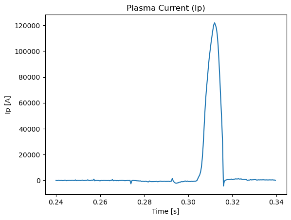
vaft.omas.plot_plasma_current_time(ods, yunit="kA")
vaft.omas.plot_pf_coil_time_current(ods, selection="active", yunit="kA")
vaft.omas.plot_flux_loop_time_flux(ods, selection="all")
vaft.omas.plot_b_field_probe_time_field(ods)
vaft.omas.plot_tf_coil_time_b_t(ods)
vaft.omas.plot_barometry_time_pressure(ods)
vaft.omas.plot_spectrometer_uv_time_intensity(ods, emission='CIII')
Every plot the registry holds – its subject, view and quantity, the adapter that draws it, and the IDS
paths it needs – is listed in the generated plot reference
(186 plots), together with the plotting functions outside the
registry: the analytic figures and the multi-shot history and scaling plots (plot_scaling_fit,
plot_H_factor_distribution, …). The page is rebuilt from vaft.plot on every publish.
The Magnetics page shows several of these traces rendered from real shots.
vaft.code
Adapters for the external codes that VAFT drives. They all share one shape: a *Config (paths,
executable, run options), an *Inputs object produced by prepare_*, a run_* that executes the
code, and a collect_* / *Result pair that reads the outputs back.
When a configuration does not supply an executable explicitly, adapters follow the documented
installation roots: EFITHOME, CHEASEHOME, GPECHOME, TESHOME, and NUBEAMHOME. Missing
binaries are a readiness state, not a failure of deterministic input preparation.
from vaft.code import EFITConfig, prepare_efit_inputs, run_efit, collect_efit_outputs

cfg     = EFITConfig(...)
inputs  = prepare_efit_inputs(ods, cfg)      # k-file and constraint set
result  = run_efit(inputs, cfg)              # EFITResult
outputs = collect_efit_outputs(workdir, cfg)
The configuration, input, result and runner types of every adapter – EFIT, CHEASE, GPEC, TES,
NUBEAM, TRANSP and the others – are listed with their signatures on the generated
vaft.code API page, one section per module.
run_nubeam_case(input_dir, gfile=..., workdir=...) is the NUBEAM equivalent: it stages a case,
builds its Plasma State, and runs INIT then STEP. Results come back as a native container, and
vaft.machine_mapping.core_sources.core_sources_from_nubeam maps the heating, current-drive and
torque channels into core_sources as an NBI source term. Heating and torque are per-zone
integrals that map directly; the driven current is not – NUBEAM reports it as a toroidal
current and IMAS asks for <J.B>/B0, so it goes through
vaft.process.equilibrium.parallel_current_from_toroidal, which needs equilibrium geometry and
assumes the driven current is field-aligned. On a spherical tokamak the two differ by about a
factor of 1.5, so the distinction is not academic.
vaft.machine_mapping.distributions.distributions_from_nubeam maps the other half: the fast-ion
population itself, one distributions.distribution entry per beam species. global_quantities
there is the exact part of the whole NUBEAM mapping – summing a per-zone integral needs no
division – and it is also where NUBEAM’s toroidal driven current survives unmodified, as
current_tor, with none of the field-aligned assumption core_sources requires. It is
current_tor and not current_fast_tor because curbeam is shielded, which is exactly the
distinction IMAS draws between those two fields; the unshielded fast-ion current NUBEAM does not
publish is left absent. The fast-ion pressures are derived: NUBEAM reports eperp_beami and
epll_beami as mean energies per particle in keV, so pressure_fast_parallel is 2 n <E_par>
and pressure_fast the scalar (p_par + 2 p_perp)/3.
When a run resolves more than one beam species, the profiles NUBEAM already summed over species –
the collisional powers and torques, and the driven current – are skipped rather than repeated
into each entry, which would double-count for a consumer that adds the entries up. A multi-species
distributions IDS therefore carries the per-species population but no driven current; those
channels remain available through core_sources, which is not species-resolved and so does not
face the same ambiguity.
vaft.machine_mapping.nbi populates the static beam geometry. What has no IMAS home yet –
deposition markers, lost fast ions, the step log’s power budget – stays in the native container
and is drawn by vaft.plot.nubeam, which is why those particular views are not in the plot
catalog while nbi_profile_* are.
TRANSP is the one adapter with no *Config, no prepare_* and no run_*: VAFT reads a TRANSP run,
it does not launch one, so there is no TRANSPHOME. read_transp_output opens a <runid>.CDF
lazily — a production file holds roughly 1900 variables — and .slice(time_s) returns one time,
reporting which sample it took.
This layer keeps TRANSP’s own names, grids and units and converts nothing: NE is still per cubic
centimetre when it reaches you. Two things it does enforce, because the file makes them easy to
get wrong. A variable’s grid comes from its dimension name and never its length — X (zone centres)
and XB (zone outer boundaries) have the same length in a real run, so state.on_x("PLFLX")
raises rather than quietly handing back a boundary quantity as a centre one. And TQTOTNB is
refused by name: it is an empty placeholder — a zero-valued scalar with no radial or time axis,
declared torque-density units notwithstanding — and the total input torque is TQIN.
enclosed_torque(state) is the one place the two grids interact: TQIN is a density in
N m / cm^3 and DVOL a volume in cm^3, both zone-centre, so the product is already newton
metres and the cumulative sum lands on the zone boundaries. Pairing them once here is deliberate —
converting one to SI and not the other is a factor of a million.
refine_equilibrium(source, config=None) is the one-shot CHEASE convenience: g-file or ODS in,
refined equilibrium out. scan_tes(ods, base_config, values, param="ip0_kA") sweeps a single TES
parameter and collects every result. Snakemake rules should start with
vaft.code.init_snakemake_logger(snakemake) so that stdout and stderr land in the rule’s log file.
Execution backends
A run_* builds the command line; an execution backend launches it. A configuration that has moved
onto the shared layer accepts backend= (default None, meaning a local child process), so the same
adapter call can later run through a scheduler without its scientific API changing.
from vaft.code import LocalBackend, TESConfig, run_tes

result = run_tes(inputs, TESConfig(timeout=600, backend=LocalBackend()))
| Name | Role |
|---|---|
ExecutionRequest |
command, working directory, environment overlay, stdin, timeout, optional merged log file, resources |
ExecutionResult |
return code (None on timeout), captured output, timed_out, runtime_status (completed, timeout, queue_timeout), elapsed time, launcher (the argv actually run), log_path, job_id (scheduler backends) |
ResourceRequest |
ntasks, threads_per_task, memory_mb; the local backend applies only the thread count |
ExecutionBackend, LocalBackend, SlurmBackend, RemoteHost, RemoteSlurmBackend, resolve_backend |
the protocol, the local, Slurm and ssh+Slurm implementations, and the config lookup (falls back to $VAFT_EXECUTION_BACKEND: local, slurm or remote) |
ExecutableNotLaunchable |
raised when the operating system refuses to start the program |
A timeout is returned (timed_out=True), not raised. A program the operating system refuses to
start raises ExecutableNotLaunchable; a missing working directory stays a FileNotFoundError.
A timeout, a KeyboardInterrupt or a SIGTERM/SIGHUP stops the program’s whole process tree
(#1016); the interrupt and the signal are then raised again rather than turned into a result.
Timeout results (#1016). Every adapter below returns its own result object on a timeout; none raises. The result says:
| Field | On a timeout |
|---|---|
status |
"failed" (a property: "completed" when ok, else "failed") |
runtime_status |
"timeout": the program ran past its limit and was stopped. "queue_timeout": a scheduler job cancelled by max_wait before it started |
returncode |
None |
elapsed_s |
wall time from launch to stop [s] (set on every run, not only a timeout); for a Slurm batch job, from submission, queue wait included |
timed_out |
True for either timeout kind (a property) |
A stop well short of timeout (a scheduler’s max_wait cancelling a running job) reports the time
actually run: a batch job’s own start and termination stamps (ExecutionResult.run_s), so a long
queue wait is not reported as running time. The reason is the last line of stderr, or of the log for codes that write one, worded
"<code> timed out after N s of running" or "<code> was cancelled after waiting N s in the scheduler
queue (it never started)".
| Adapter | Timeout result | Notes |
|---|---|---|
CHEASE run_chease, refine_equilibrium |
CHEASEResult |
nothing is collected; chease.log holds the partial output and the reason |
scan_chease |
the case keeps its CHEASEResult |
case.error names the limit; the scan goes on (keep_going) |
synthesize_equilibrium_from_0d |
SyntheticEquilibriumResult |
status="timeout" with the reason, rather than non_converged |
synthesize_equilibrium_to_targets |
MultiTargetSynthesisResult |
status="chease_failed"; the reason names the solve and its timeout, and that solve’s history record keeps status="timeout" |
GACODE run_gacode |
GACODERun |
unpacks as (returncode, log) as before, with returncode=None; .runtime_status, .elapsed_s |
NEO run_neo, TGLF run_tglf |
NEOResult, TGLFResult |
check=True (the default) raises NEOExecutionError/TGLFExecutionError naming the limit, as for any failure; check=False returns it |
NUBEAM run_nubeam, run_nubeam_case |
NUBEAMResult |
a stopped INIT, STEP or Plasma State stage; generate_plasma_state returns a path, so there it raises NUBEAMExecutionError |
FLARE run_flare |
FlareResult |
|
TES run_tes, scan_tes |
TESResult |
outputs are still collected, as before |
NICE run_nice |
NiceResult |
termination_reason is the reason; the manifest records process_runtime_status |
GENRAY run_genray |
GENRAYResult |
|
| EFIT, EFUND, GPEC suite | unchanged for now | see “Previous behaviour”; they move after 2026-10-06 |
Previous behaviour (0.7.x), kept for reference:
| Adapter | What a timeout produced |
|---|---|
| TES | returncode=124 |
| EFIT | status="failed", runtime_status="timeout" |
| EFUND | failed, returncode=None |
| GPEC suite | GPECModuleRun: completed if its core outputs verify, else failed/None |
scan_chease |
an error string per case ("TimeoutExpired: ...", result=None) |
| NICE, GENRAY | returncode=124 |
| CHEASE, GACODE (NEO, TGLF), NUBEAM, FLARE | raised subprocess.TimeoutExpired |
Every adapter that runs a subprocess goes through the backend, and each has a backend field:
EFIT and EFUND, CHEASE, TES, the GPEC suite, GACODE (NEO and TGLF), NUBEAM, FLARE and NICE. CodeConfig
carries the field too. EFIT and EFUND declare one thread per task (threads_per_task=1), which sets
OMP_NUM_THREADS, MKL_NUM_THREADS, OPENBLAS_NUM_THREADS, VECLIB_MAXIMUM_THREADS and
NUMEXPR_NUM_THREADS to 1 unless the environment already sets them. GACODE
declares n_mpi and FLARE declares processes as ntasks for scheduler backends, while their
launchers still start the ranks themselves. TokaMaker runs in-process and has no backend.
Running under Slurm
SlurmBackend (#1017) runs the same adapter call as a cluster job. Only the backend= argument
changes:
from vaft.code import EFITConfig, SlurmBackend, run_efit

config = EFITConfig(timeout=1800, backend=SlurmBackend(partition="short", account="vest"))
result = run_efit(inputs, config)          # same EFITResult as a local run
Modes. The backend picks one of two automatically. Pass mode="step" or mode="batch" to force it.
- Step (inside an allocation, i.e.
SLURM_JOB_IDis set). The command runs as a job step withsrun. The timeout is enforced twice: assrun --time, and as a local deadline after whichsrunis interrupted so that it cancels the step. Ifsrunstill does not exit, it is killed and its step is cancelled by its unique name. The local deadline starts at launch, so time spent waiting for step resources counts against it. The backend adds--overlapwhen the caller is itself running in a step. It also leaves out the step defaults the caller inherited from an enclosing step or job: CPU and memory binding, distribution, per-task CPUs and GPUs, and, when--memis requested, the per-CPU memory setting. Values that you set in the request’senv, or pass throughextra_args(for example--cpu-bind=none), are kept. - Batch (everywhere else). The backend writes a job script with mode 0700 under
<workdir>/.vaft-slurm/, submits it withsbatch --parsable --no-requeue, and pollssqueueuntil the job is no longer live. The script records the program’s exit status itself, so the backend does not needsacct. Whensacctis available, the backend uses it to refine the job state.
Resources. Both modes request --nodes=1 --ntasks=1 --cpus-per-task=<ntasks x threads>.
ResourceRequest.ntasks counts the ranks that a self-launching program (GACODE, FLARE) starts
itself, and those ranks have to fit inside that single task. Each MPI launcher integrates with
Slurm differently, so test each such code on a real cluster before relying on it.
Timeouts.
timeoutbecomes the walltime (--time), rounded up to whole minutes.timeout=Nonesends no--time, so the partition’s default walltime applies.- A job that Slurm ends as
TIMEOUTreturnstimed_out=True. Withoutsacct, the backend infers this on the node: fromSLURM_JOB_END_TIMEwhere Slurm sets it, otherwise from the runtime compared with the requested walltime, less one minute for the prolog. max_waitcaps the total time the backend blocks, including time in the queue. After that the job is cancelled, and the reason is written tostderror appended to the log. A job cancelled before its program started reportsruntime_status="queue_timeout"; one cancelled while running,"timeout".
Other outcomes.
- If
sbatchorsrunis missing, or Slurm rejects the submission, the backend raisesExecutableNotLaunchable. - A job that ends without the program finishing (cancelled, node failure, preemption, out of memory)
gets a non-zero
returncode, and its Slurm state is appended tostderror to the log. - An executable that exists on the login node but not on the compute node shows up as exit status 127.
KeyboardInterruptwhile waiting cancels the job.
Environment. The job script exports only the environment entries that differ from the
submitting process; --export=ALL carries everything else. The backend never exports SLURM_*,
SBATCH_* or SRUN_* variables, and never exports names that are not valid shell identifiers.
Shared filesystem. The working directory and the executables must be on a filesystem that the compute nodes share. The backend does not check this.
Switching everything at once. Setting VAFT_EXECUTION_BACKEND=slurm moves every adapter that
names no backend onto Slurm. Placement comes from VAFT_SLURM_PARTITION, VAFT_SLURM_ACCOUNT,
VAFT_SLURM_QOS, VAFT_SLURM_MODE and VAFT_SLURM_MAX_WAIT. This setting also queues short runs
such as EFUND or a single EFIT slice, so prefer an explicit backend= for those.
Running on a cluster over ssh
SlurmBackend submits from a host that can run sbatch itself. When the machine that prepares a
case is not the machine that can run it – a laptop holding the inputs, a cluster holding the build
– RemoteSlurmBackend does the same job over ssh:
from vaft.code import RemoteHost, RemoteSlurmBackend
from vaft.code.gpec import GPECSuiteConfig

host = RemoteHost(
    host="login.example.org",
    user="me",
    work_root="/scratch/me/vaft",
    # Ordered local -> remote prefix pairs; the first match at a path boundary wins.
    path_maps=(("/opt/gpec", "/apps/gpec/1.4"),),
    setup_lines=("module purge", "module load gpec/1.4"),
    fetch=("*.nc", "*.out"),          # "all" (default), "none", or glob patterns
)
config = GPECSuiteConfig(
    timeout=7200,
    backend=RemoteSlurmBackend(host, partition="short", account="fusion", max_wait=43200),
)
One run rsyncs the working directory up, writes the same job script SlurmBackend writes (with
setup_lines in front), submits it with ssh … sbatch --parsable --no-requeue, polls squeue and
then sacct over ssh with a growing interval, and rsyncs back what the fetch policy names. The
result is the one a local run returns: the same timeout and queue_timeout statuses, the same
ExecutableNotLaunchable for a refused submission, and run_s taken from the scheduler’s start and
end stamps. KeyboardInterrupt, SIGTERM and SIGHUP scancel the job and are then raised again.
Paths. The two machines share no filesystem, so the working directory, log_path, every
command argument (--home=/opt/gpec included) and every path-valued env entry go through
path_maps. A working directory that no pair covers is staged into a fresh directory under
work_root. A prefix matches only at a path boundary, so /data/runs2 is not under /data/runs.
Environment. --export=ALL carries the host’s ssh environment, not the laptop’s, which is the
point: the job’s search paths come from the host’s login environment and from setup_lines. Only
the request’s own entries travel, path-translated, and the ones whose value describes the submitting
machine never do – PATH, LD_LIBRARY_PATH, DYLD_*, PYTHONPATH, HOME, TMPDIR, the locale
and the loaded-module state (vaft.code.remote.UNFORWARDED_ENVIRONMENT). A macOS PATH on a Linux
compute node would shadow exactly what the modules just set up.
What comes back, and what stays. The job log and the scratch directory always come back; the
fetch policy governs the rest of the working directory, so a run with tens of GB of output can
leave it on the cluster and bring back an extract. The host’s copy is kept by default
(keep_remote=True) because it is usually the only full copy; keep_remote=False removes it after
the fetch, and only ever a directory the backend staged under work_root.
Credentials. None are handled here. ssh always runs with BatchMode=yes, so a host that would
prompt fails at once instead of blocking a batch; keys and agents are yours to arrange. Pass extra
ssh arguments through ssh_options, and a key file through identity_file.
Switching everything at once. VAFT_EXECUTION_BACKEND=remote builds the backend from
VAFT_REMOTE_HOST, VAFT_REMOTE_WORK_ROOT (both required), VAFT_REMOTE_USER,
VAFT_REMOTE_PORT, VAFT_REMOTE_IDENTITY, VAFT_REMOTE_SSH_OPTIONS, VAFT_REMOTE_PATH_MAPS
(local=remote pairs, comma separated), VAFT_REMOTE_SETUP (; separated), VAFT_REMOTE_FETCH
and VAFT_REMOTE_KEEP, plus the same VAFT_SLURM_PARTITION, VAFT_SLURM_ACCOUNT,
VAFT_SLURM_QOS and VAFT_SLURM_MAX_WAIT a local submission reads. Every call then costs at least
two ssh round trips and two rsyncs, so keep short runs (EFUND, one EFIT slice) on an explicit local
backend=.
In-process memory guard
ResourceRequest.memory_mb only asks a scheduler for memory, and LocalBackend ignores it. When a
long Python loop outgrows its allocation, the kernel’s or Slurm’s OOM killer ends the process with no
traceback and no status record. vaft.code.resources (#1146) lets the loop notice first and stop at a
point of its own choosing:
from vaft.code import MemoryBudget, MemoryBudgetExceeded, memory_budget, peak_rss_mb, rss_mb

budget = memory_budget()                    # MemoryBudgetInfo(limit_mb, source, candidates, ...)
with MemoryBudget(budget, fraction=0.9, interval_s=0.5) as guard:   # or limit_mb=None to resolve on entry
    for item in range(3):
        try:
            guard.check(label=item)         # raises above 0.9 x limit_mb
        except MemoryBudgetExceeded as error:
            print(f"stopping at {error.label}: {error.rss_mb:.0f} MiB")
            break
print(guard.peak_mb, rss_mb(), peak_rss_mb())
| Name | Role |
|---|---|
rss_mb(), peak_rss_mb() |
current and process-lifetime peak resident set size, MiB |
memory_budget(environ=None) |
the effective limit: the minimum of the sources below, with the one that set it |
MemoryBudgetInfo |
limit_mb (None when nothing reports a limit), source, every candidates value; as_dict() for status files |
MemoryBudget(limit_mb=None, fraction=0.9, *, on_exceed="raise", interval_s=None) |
context manager; limit_mb is MiB or a MemoryBudgetInfo; check(label), peak_mb, start_interval() and interval_peak_mb (the peak of one loop item), exceeded, as_dict() |
MemoryBudgetExceeded |
a MemoryError (so an except RuntimeError around one item does not swallow it; code that catches MemoryError to fall back to a chunked path will, so re-raise it there); picklable across a process pool; rss_mb (the memory in use observed), threshold_mb, limit_mb, label, source, peak_mb |
cgroup_usage_mb(directory, kind) |
a cgroup’s non-reclaimable usage (anon + shmem; v1 total_rss + total_shmem), MiB |
Sources, all in MiB (2**20 bytes, which is what Slurm means by MB):
source |
Value |
|---|---|
slurm_mem_per_node |
SLURM_MEM_PER_NODE |
slurm_mem_per_cpu |
SLURM_MEM_PER_CPU × SLURM_CPUS_ON_NODE |
cgroup_v2 |
memory.max, the smallest from the process’s cgroup up to the root, since Slurm puts the limit on the job cgroup and runs the process in a step below it |
cgroup_v1 |
memory/…/memory.limit_in_bytes, likewise; the unlimited sentinel is ignored |
env |
VAFT_MEMORY_BUDGET_MB; it can lower the budget, never raise it past another source |
mem_available |
this process’s RSS plus MemAvailable at call time (psutil, or vm_stat on macOS, off Linux): what the process could grow to; other processes may take it first |
RLIMIT_AS is not a source: it limits address space, which numpy reserves far ahead of what it
touches, so MemoryError arrives at that limit with RSS far below it and no RSS guard can see it.
The guard. limit_mb=None resolves the budget with memory_budget() on entry. When nothing
reports a limit, the guard only records peak_mb. check() compares the memory in use with
fraction × limit_mb: this process’s RSS, or, when a cgroup set the limit, the larger of that and the
cgroup’s non-reclaimable usage, because the cgroup’s limit also counts child processes, sibling tasks
and tmpfs (page cache is left out: the kernel drops it before the OOM killer runs). Entering a guard
again starts afresh. With interval_s, a daemon thread also samples RSS; a crossing it sees sets a
flag, and the next check() raises even if RSS has fallen since, so a single large numpy call between
two checks is still caught. The thread never raises into the caller. Leaving the block never raises
either: a crossing that no check() reported stays in exceeded. on_exceed="warn" issues one
ResourceWarning and records the event instead of raising. peak_mb is the largest RSS the guard
saw, a lower bound on the true peak inside the block; peak_rss_mb() is the process’s lifetime peak.
Platforms. Linux reads VmRSS/VmHWM from /proc/self/status. macOS reads the current RSS with
task_info and the peak with getrusage, whose ru_maxrss is in bytes there and in KiB on Linux.
Windows reads GetProcessMemoryInfo. psutil is used when it is installed and no native reading is
available, and ps -o rss= is the last resort; psutil is never required. The guard stops the Python
process only; it does not limit LocalBackend children (see #1016).
vaft.data
Portable file formats and the packaged sample files.
from vaft.data import read_geqdsk, write_geqdsk, to_omas, from_omas, sample_geqdsk, data_path

geq = read_geqdsk("g039915.00319")          # GEQDSK
ods = to_omas(geq)                          # GEQDSK to ODS (equilibrium IDS)
geq = from_omas(ods, time_index=0)          # ODS to GEQDSK
write_geqdsk(geq, "g039915.00319.copy")

geq  = sample_geqdsk()                      # packaged default: efit/g039915.00319
root = data_path()                          # the packaged vaft/data directory
from_imas and to_imas perform the same round trip against a native IMAS entry instead of an ODS.
vaft.imas
Local IMAS artifacts: vaft.imas.save writes an ODS, a native IDS or an IMASHandle to an IMAS HDF5
directory or .nc file, and vaft.imas.load opens one as a native DBEntry context manager.
IMAS_DD_VERSION_CONVERSION is the Data Dictionary version used for conversion, overridable through the
environment variable of the same name. The OMAS-derived Access Layer bridge underneath — load_omas_imas,
save_omas_imas, imas_open, imas_open_uri, imas_get, imas_set — lives in vaft.imas.omas_imas.
vaft.database uses this under the hood; call it directly only when you need to talk to an Access
Layer entry that is not a VEST shot. See
Data structures for worked examples.
Notebooks and workflows
Each subpackage has at least one notebook that exercises it end to end:
| Area | Notebook |
|---|---|
vaft.database |
database_initialization_and_load.ipynb |
vaft.database.raw |
vest_raw_signal_sql_database.ipynb |
vaft.data, vaft.imas |
imas_omas_data_conversion.ipynb, read_and_convert_data_structure.ipynb |
vaft.machine_mapping, vaft.process.magnetics |
magnetic_diagnostics_processing.ipynb |
vaft.process.electromagnetics |
electromagnetic_response_modeling_with_efund.ipynb, eddy_current_calculation_and_startup_analysis.ipynb |
vaft.code |
magnetic_equilibrium_reconstruction_with_efit.ipynb, equilibrium_refinement_using_chease.ipynb, perturbed_equilibrium_and_3d_response_with_gpec.ipynb, forward_equilibrium_using_TES.ipynb, vest_nbi_analysis_with_nubeam.ipynb |
vaft.formula, vaft.process.statistical_analysis |
confinement_time_scaling.ipynb, tokamak_power_balance.ipynb |
vaft.plot |
plotting_sample_using_vaft_plot_module.ipynb |
The Snakemake pipelines that stitch these together live under
workflow/:
automatic_pipeline_1_routine_data_processing (raw DAQ to diagnostics ODS to constraints to EFIT and
CHEASE), automatic_pipeline_2_corrective_data_update (re-run equilibrium and profile updates on
existing shots), and automatic_pipeline_3_data_summary (multi-shot history tables and figures).
Source
Browse the package on GitHub: vaft/ —
database/,
omas/,
process/,
formula/,
machine_mapping/,
plot/,
code/,
data/,
imas/.
See also
- Quick start guide — install, connect, load a shot.
- Data structures — ODS, IDS and the IMAS data model.
- Signal processing and EM modeling —
vaft.processin depth. - Formula reference — every
vaft.formulafunction with definition, units, conventions and references. - Magnetics — plotting the magnetics IDS.
- Examples — the notebook index.
What these objects mean scientifically – which concept a plot draws, which diagnostic measures it, which Data Dictionary path represents it – is generated in the scientific ontology explorer.