Geometric approximations
Analytic tokamak theory seldom works in the real torus. It works in a slab, a cylinder or an expanded
torus, and it carries a few coefficients over from the real equilibrium. This page sets out those
reductions using the literature’s names. The formulas are in
vaft.formula.geometry.
The toroidal parent geometry itself (flux surfaces, the Shafranov shift, shaping, $q$ as a winding number, and $\theta$ versus $\theta^*$) is drawn in the tokamak-geometry section of Scientific diagrams. How VAFT keeps coordinates, projections, representations, derived quantities and solver conventions of one real equilibrium apart is on Equilibrium representations.
Two axes, not one hierarchy
Geometry says what space the model lives in: slab, cylindrical or toroidal. Ordering says which scales are assumed small: local ($|x| \ll r$), large aspect ratio ($\epsilon = a/R_0 \ll 1$) or neither (global). The two are independent. A slab may carry $q$, $\hat s$, $R_0$ or a $1/R_0$ curvature inherited from a torus and still be a slab. Large aspect ratio is an ordering, not a geometry: some large-aspect-ratio theories stay toroidal.
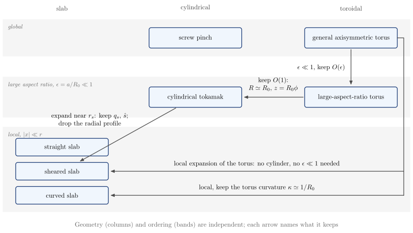
| Representation | Geometry | Typical ordering | Retained | Neglected or parameterized |
|---|---|---|---|---|
| straight slab | slab | local | local gradients, wave propagation | curvature, magnetic shear |
| sheared slab | slab | local | local gradients, magnetic shear, resonance | global geometry; curvature unless added |
| curved slab | slab | local | shear plus a prescribed curvature, e.g. $1/R_0$ | global toroidal geometry |
| cylindrical tokamak | cylindrical | large aspect ratio, leading order | radial structure, current profile, $q(r)$, rational surfaces | toroidicity, shaping |
| large-aspect-ratio torus | toroidal | $\epsilon \ll 1$ | selected $O(\epsilon)$ toroidal corrections | higher orders in $\epsilon$ |
| general axisymmetric torus | toroidal | global | shaping, curvature, toroidal coupling | nothing geometric |
Conventions used throughout
- Perturbations are $e^{i(m\theta - n\phi)}$, as in
vaft.formula.helical_phase. Both mode numbers are positive and the helicity is in the minus sign. - $q$ is a magnitude, whatever sign a COCOS gives it. $\hat s$ keeps the sign of $d|q|/dr$: reversed shear ($\hat s < 0$) flips the sign of $L_s$.
- A torus is straightened at $R_0$ with $z = R_0\phi$ and $B_z \leftrightarrow B_\phi$. Along that $z$, the harmonic has wavenumber $-n/R_0$.
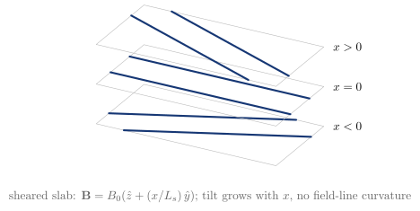
- A sheared slab is $\mathbf B = B_0(\hat{\mathbf z} + (x/L_s)\hat{\mathbf y})$, with $z$ along the field at $x = 0$ and $y$ the binormal in the surface. This field-aligned $z$ is not the straightened-torus $z = R_0\phi$.
- The local slab of a surface $r_0$ is that frame, with $x = r - r_0$. There the harmonic has:
- $k_y = m/r_0$;
- $k_z = (m - nq_0)/(q_0R_0)$, which is zero on a rational surface;
- $L_s$, which is signed: positive shear gives $L_s = -q_0R_0/\hat s < 0$.
local_slab_from_cylinderreturns $(k_y, L_s, k_z)$ in the ordersheared_slab_parallel_wavenumbertakes them.shear_length_from_q_R0_sreturns the magnitude $qR_0/|\hat s|$.
Straight slab
- Coordinates: $(x, y, z)$: radial, binormal, along $\mathbf B$.
- Field: $\mathbf B = B_0\hat{\mathbf z}$, uniform.
- Ordering: local. Gradients are taken over a region small against every equilibrium scale.
- Formula: $\tilde f \propto e^{i(k_xx + k_yy + k_zz)}$, and $k_\parallel = \mathbf k\cdot\mathbf B/B = k_z$
(
slab_parallel_wavenumber). - Keeps: wave propagation and local density or temperature gradients.
- Drops: magnetic curvature and magnetic shear, unless they are added separately.
- Used for: drift waves, and local dispersion relations before shear or curvature enter.
Sheared slab
- Field: $\mathbf B = B_0(\hat{\mathbf z} + (x/L_s)\hat{\mathbf y})$ (
sheared_slab_field), or equivalently $B_y(x) \simeq B_y’x$ near a resonant surface. - Shear: $\hat s = (r/q)\,dq/dr$ (
vaft.formula.shear_from_r_q). Under the local, large-aspect-ratio ordering, $|L_s| = qR_0/|\hat s|$ (shear_length_from_q_R0_s). - Formula: $k_\parallel(x) \simeq k_z + k_y x/L_s$ (
sheared_slab_parallel_wavenumber). The perturbation is field-aligned on one surface and $|k_\parallel|$ grows linearly away from it. - Keeps: the resonance and its localisation.
- Drops: global geometry, and curvature unless it is added.
- Used for: the inner layer of tearing modes (FKR, Rutherford), drift waves with shear, and the local limits of gyrokinetics.
- Related configurations in the same frame: the reversing field of a Harris current sheet,
$B_y = B_0\tanh(x/a)$ (
harris_sheet_field,harris_sheet_current_density), whose centre is a sheared slab with $B_y’ = B_0/a$ and no guide field, and the current-free X-point $\psi = B’(x^2 - y^2)/2$ (x_point_flux). These configurations, not geometries, are drawn in the field-configuration section of the diagrams guide.
Curved slab
Curved slab is a family of local models, not one model. VAFT fixes no closure here: the curvature coefficient is whatever a particular model inherits from its parent torus.
- Coordinates and field: those of the straight or sheared slab.
- Curvature: toroidal curvature is added as a parameter, either an effective curvature $\boldsymbol\kappa = \mathbf b\cdot\nabla\mathbf b$ (typically $|\kappa| \simeq 1/R_0$ pointing to the major axis), or an effective gravity $g \sim v_{th}^2/R_0$.
- Ordering: local. The curvature is a constant coefficient over the region.
- Keeps: the interchange drive (the pressure gradient against the curvature) and the $\nabla B$ and curvature drifts.
- Drops: the poloidal variation of curvature (good and bad curvature sides), the geometry of the real flux surfaces, and toroidal mode coupling.
- Next more realistic model: a local toroidal (flux-tube) model, where $\kappa$ varies along the field line.
- Used for: interchange and Rayleigh–Taylor analogues, resistive-g modes, and reduced edge and SOL turbulence.
Cylinder, screw pinch, cylindrical tokamak
- Coordinates: $(r, \theta, z)$.
- Field: $\mathbf B = B_\theta(r)\hat{\boldsymbol\theta} + B_z(r)\hat{\mathbf z}$.
- Safety factor: $q(r) = rB_z/(R_0B_\theta)$ (
cylindrical_safety_factor_from_r_B). - Resonance: $k_\parallel = (m - nq)/(qR_0)$ (
cylindrical_parallel_wavenumber), so $k_\parallel = 0 \Leftrightarrow q(r_s) = m/n$. - The three are related but not synonyms:
- A straight cylinder is only the coordinate system.
- A screw pinch is a cylindrical equilibrium with both $B_\theta(r)$ and $B_z(r)$, so its field lines are helices. Pure $\theta$- and $z$-pinches are its limits.
- A cylindrical (straight) tokamak is a screw pinch that is periodic in $z$ with length $2\pi R_0$ and has $B_z \gg B_\theta$, both taken from a torus.
- Keeps: radial structure, the current profile, $q(r)$ and rational surfaces.
- Drops: $1/R$ variation of $B_\phi$, toroidal curvature, inboard/outboard asymmetry, the Shafranov shift, toroidal coupling of harmonics, and shaping. The helical field lines are still curved, which is what drives Suydam interchange.
- Used for: Newcomb’s equation, the internal kink, the outer tearing problem and $\Delta’$.
Large-aspect-ratio ordering
For a circular torus $R = R_0 + r\cos\theta$, so
\[\frac{1}{R} = \frac{1}{R_0}\left[1 - \frac{r}{R_0}\cos\theta + O(\epsilon^2)\right],\qquad B_\phi = B_0\frac{R_0}{R} = B_0\left[1 - \frac{r}{R_0}\cos\theta + O(\epsilon^2)\right].\]The second expression is vaft.formula.vacuum_toroidal_field.
Worked $O(\epsilon)$ example: toroidal coupling. Any factor of $1/R$ multiplying a harmonic $e^{im\theta}$ creates sidebands:
\[\frac{e^{im\theta}}{R} = \frac{1}{R_0}\left[e^{im\theta} - \frac{\epsilon}{2}\left(e^{i(m+1)\theta} + e^{i(m-1)\theta}\right)\right] + O(\epsilon^2),\qquad \epsilon = r/R_0 .\]So in a torus an $m/n$ perturbation drags along $(m \pm 1)/n$ components of relative size $\epsilon/2$. In a cylinder it cannot.
The expansion is used in two different ways:
- Large-aspect-ratio toroidal model. It keeps selected $O(\epsilon)$ terms:
- curvature;
- inboard/outboard asymmetry;
- coupling of $m$ to $m \pm 1$.
It is still toroidal. It keeps the $O(\epsilon)$ curvature and $1/R$ terms and drops $O(\epsilon^2)$. The Shafranov shift enters at $O(\epsilon(\beta_p + l_i/2))$ relative to $a$. Shaping is outside the circular expansion used here, although shaped large-aspect-ratio models exist (for example Miller local equilibria). Typical uses are the $s$–$\alpha$ ballooning model, toroidal Alfvén gaps and neoclassical trapping.
- Cylindrical tokamak limit. It keeps only $O(1)$: $R \simeq R_0$, and the toroidal direction is straightened as $z = R_0\phi$. The cylindrical tokamak is the leading-order limit of the large-aspect-ratio expansion. It is not the same thing as large aspect ratio.
Local sheared-slab reduction
Near a surface $r_0$, with $x = r - r_0$ and $|x| \ll r_0$, expand $q \simeq q_0 + q_0’x$ and take the field-aligned frame: $z$ along $\mathbf B(r_0)$, $y$ the binormal. The harmonic $e^{i(m\theta - n\phi)}$ has there
\[k_y = \frac{m}{r_0},\qquad L_s = -\frac{q_0R_0}{\hat s},\qquad k_z = \frac{m - nq_0}{q_0R_0}\](local_slab_from_cylinder). Along the straightened torus the same harmonic has $-n/R_0$; along the
field it has $k_z$. On a rational surface $q_0 = m/n$, so the resonance $q(r_s) = m/n$ becomes
$k_\parallel(0) = k_z = 0$ and the shear becomes $k_\parallel’ = k_y/L_s = -k_y\hat s/(q_0R_0)$. The test
suite checks that this slab reproduces the cylinder’s $k_\parallel$ to first order in $x$.
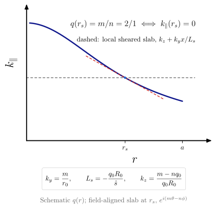
A local slab does not need a cylinder as an intermediate step. It can be expanded from a toroidal equilibrium directly. What defines it is locality relative to the equilibrium scale, not large aspect ratio. Turbulence and interchange models often keep toroidal coefficients in a slab, such as $|L_s| \simeq qR_0/|\hat s|$ and, in curved slabs, $\kappa \simeq 1/R_0$.
The same field line in each geometry
| Toroidal | Cylindrical | Sheared slab |
|---|---|---|
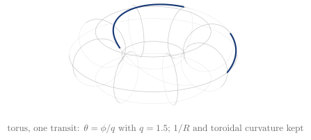 |
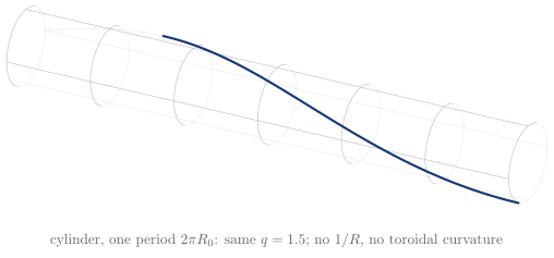 |
 |
MHD mode representations across geometries
The same instability is described differently in each geometry, and MHD vocabulary mixes several classification systems in one name. “$m = 1$”, “kink”, “internal”, “ideal”, “tearing parity”, “low-$n$” and “resonant” are answers to different questions. Schematically,
\[\text{mode} = \text{spectral label} + \text{drive} + \text{localisation} + \text{resonance} + \text{parity} + \text{physical model},\]and two modes with the same name can differ in any of these. This section maps mode families across the slab, cylindrical and toroidal reductions above. It does not claim that every mode has a unique descendant in the next geometry.
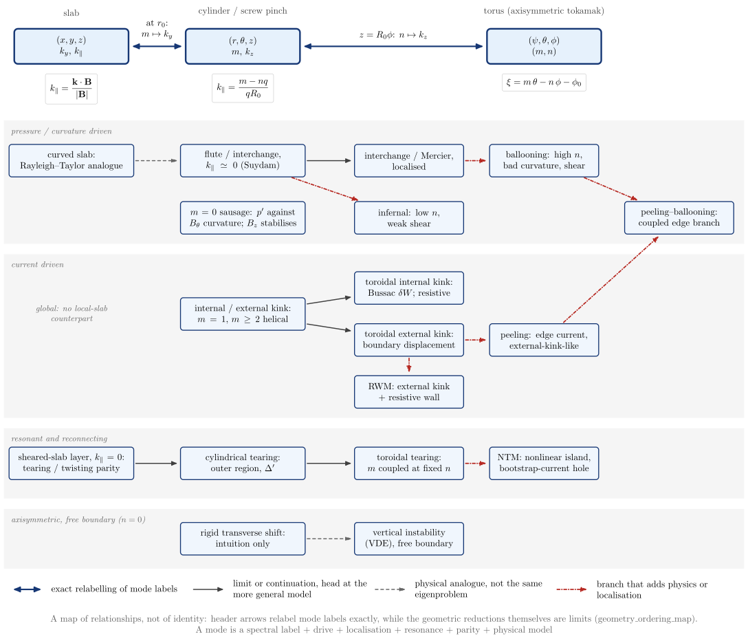
mhd_mode_geometry_map keeps four kinds of relation apart, and draws each with its own arrow:
| Relation | Meaning | Example |
|---|---|---|
| exact relabelling | the same harmonic’s labels in another geometry’s coordinates; the geometric reduction behind it is still a limit (geometry_ordering_map) |
$n \mapsto k_z = -n/R_0$ along $z = R_0\phi$; $m \mapsto k_y = m/r_0$ at a surface $r_0$ |
| limit or coordinate continuation | one description is a limit of the other; the arrowhead points at the more general model | Suydam’s criterion is the cylindrical limit of Mercier’s |
| physical analogue | the same mechanism in a different eigenproblem | magnetic Rayleigh–Taylor and interchange |
| branch | extra physics or localisation on top of a family | a resistive wall turns the external kink into an RWM |
Fourier representation and resonance
With the conventions above, a perturbation is
| Geometry | Representation | Spectral labels |
|---|---|---|
| slab | $\tilde f \propto e^{i(k_xx + k_yy + k_zz)}$ | $k_y$, $k_\parallel = \mathbf k\cdot\mathbf B/B$ (slab_parallel_wavenumber) |
| cylinder | $\tilde f \propto e^{i(m\theta + k_zz)}$ | $m$, $k_z$ |
| torus | $\tilde f \propto e^{i(m\theta - n\phi)}$ | $(m, n)$, phase $m\theta - n\phi$ (helical_phase) |
Straightening the torus at $R_0$ gives $z = R_0\phi$ and $k_z = -n/R_0$. The field-aligned local slab of
a surface (local_slab_from_cylinder) has $k_y = m/r_0$, and along the field the harmonic has
$k_\parallel = (m - nq)/(qR_0)$ (cylindrical_parallel_wavenumber). Hence
which is mode_number_mapping. These relations exist once, in vaft.formula.geometry and
vaft.formula.stability.helical_phase; the map quotes them and implements nothing new.
Mode numbers are morphology, not instability
In a cylinder, $m = 0$ is a sausage, $m = 1$ a kink (a rigid helical shift) and $m \ge 2$ higher helical
distortions (cylindrical_mode_morphology). These are Fourier morphologies. They are not a
taxonomy of instabilities. “$m = 1$ means kink instability” says too much. It is more accurate to say that
$m = 1$ has kink-like cylindrical morphology, and that whether an unstable kink branch exists depends on
the equilibrium and on the eigenproblem posed. The $m = 0$ sausage instability of a Z-pinch is driven by
the pressure gradient against the curvature of $B_\theta$, so the map files it under the pressure-driven
family. A strong $B_z$ stabilises it, and it has no tokamak descendant on the map.
Pressure- and curvature-driven family
\[\text{Rayleigh–Taylor analogue} \to \text{flute / interchange} \to \text{interchange / Mercier, ballooning, infernal}\]- Curved slab. A pressure gradient against a prescribed field-line curvature acts like a heavy fluid above a light one, with the curvature playing gravity: a magnetic Rayleigh–Taylor analogue.
- Cylinder. Flute or interchange perturbations have $k_\parallel \simeq 0$ and so bend field lines as little as possible. Suydam’s criterion is their local stability limit. Interchange names a mechanism, not a mode number.
- Torus. Three branches are kept apart:
- interchange / Mercier: the localised pressure–curvature limit; Mercier’s criterion is the toroidal continuation of Suydam’s;
- ballooning: high $n$, modified by field-line bending and magnetic shear and localised on the
bad-curvature side (
ballooning_curvature_drive,ballooning_harmonic_envelope,ballooning_eigenfunction,s_alpha_ballooning); - infernal: low $n$, pressure-driven, where magnetic shear is weak.
Current-driven family
The internal/external distinction already exists in the cylinder (internal_external_kink;
Kruskal–Shafranov is a cylindrical external-kink criterion). The torus continues both:
- Internal kink: a global ideal mode confined inside an internal rational surface, the $m = 1$ mode inside $q = 1$. In a torus its leading cylindrical $\delta W$ vanishes and the toroidal (Bussac) terms decide stability. Finite resistivity at $q = 1$ gives the resistive kink.
- External kink: a global ideal mode that displaces the plasma boundary (
internal_external_kink,plasma_vacuum_wall,kink_mode). - Peeling: an edge-current-driven, edge-localised, external-kink-like branch. It is not simply the same mode as the external kink.
- Resistive-wall mode (RWM): the external-kink branch modified by a finite-conductivity wall. It grows on the wall time instead of the Alfvén time.
- Peeling–ballooning: the coupled edge branch of peeling and ballooning, the picture behind the
peeling_ballooningoperational diagram.
Global current-driven modes have no local-slab counterpart. They need the radial current profile that a local slab discards.
Resonant and reconnecting family
global toroidal / cylindrical harmonic
  -> q = m/n                          (mode_number_mapping)
  -> cylindrical ideal outer problem  (cylindrical_tearing_outer, Delta')
  -> local sheared-slab layer         (slab_parity, rational_surface)
  -> tearing or twisting channel      (resonant_layer_matching, tearing_layer_matching)
The tearing mode is the resistive resonant instability. In a torus, toroidicity and shaping couple
several $m$ at fixed $n$ (poloidal_harmonic_coupling), so the outer problem becomes a matrix over all
rational surfaces of that $n$. The NTM is a nonlinear, neoclassical extension of island evolution,
driven by the loss of bootstrap current inside the island (magnetic_island). It is not the next linear
eigenmode in an ideal–resistive hierarchy, which is why it hangs off the map as a branch.
Parity is orthogonal to mode number
$m$ and $n$ are not parity labels. At a resonant surface the local layer response has its own
classification, tearing or twisting parity (slab_parity, slab_parity_comparison). A given
$m/n$ harmonic can take part in either channel, depending on the response or eigenproblem. Toroidal
coupling of several $m$ at fixed $n$ does not change this. Parity stays a separate concept. With finite
pressure and curvature, the Glasser–Greene–Johnson inner layer that RDCON solves classifies its solutions
as tearing and interchange parity rather than twisting.
Axisymmetric free-boundary modes
The vertical instability, and the VDE it leads to, is $n = 0$, axisymmetric, and set by elongation and the
free boundary (hot_vde_sequence, cold_vde_bifurcation, vde_timescales). It does not belong to the
kink family. A rigid transverse shift of a cylinder is useful intuition and nothing more. There is no
exact $m = 1 \leftrightarrow$ VDE equivalence.
Orthogonal mode descriptors
| Descriptor | Examples | What it tells us |
|---|---|---|
| geometry | slab, cylinder, torus | the space the model lives in |
| spectral label | $k_y, k_\parallel$; $m, k_z$; $(m, n)$ | Fourier structure |
| drive | pressure and curvature, current, bootstrap current | the free-energy source |
| localisation | core, internal, global, edge | radial structure |
| resonance | resonant, non-resonant | relation to $k_\parallel = 0$ |
| parity | tearing, twisting | local layer symmetry |
| model | ideal, resistive, neoclassical, wall-coupled | the physics retained |
| ordering | $n = 0$, low $n$, intermediate $n$, high $n$ | spectral and asymptotic regime |
Where VAFT’s stability tools sit
| Tool | Place on the map |
|---|---|
analytic criteria (vaft.formula.stability) |
Mercier- and interchange-like limits, ballooning limits, operational boundaries |
| DCON | finite-$n$ ideal MHD: global ideal mode structure and the energy principle |
| RDCON / STRIDE | resonant outer regions matched to inner layers: tearing and twisting channels |
| GPEC | the forced, perturbed 3-D response: resonant and non-resonant harmonics |
These tools do not share a common “instability severity” scale. Interchange, ballooning, kink and peeling should not be ranked by comparing unrelated criteria with each other. Naming the dominant dynamical mode needs a common eigenvalue or growth-rate problem. How VAFT runs these codes is on MHD stability.
Gyrokinetic micro-instabilities (ITG, TEM, ETG, MTM, KBM) are outside this MHD map. They can use the same coordinate framework later.
Where these lead
cylinder / screw pinch  -> Newcomb equation, internal kink, outer tearing (Delta')
cylinder -> sheared slab -> resistive inner layer: FKR, Rutherford, modified Rutherford
straight / sheared / curved slab -> drift waves, interchange, reduced edge turbulence, local gyrokinetics
The tearing diagrams (rational_surface, delta_prime, tearing_layer_matching) start from the
cylinder and sheared slab described here. The current-sheet, X-point, reconnection and MHD-wave
diagrams (current_sheet, x_point, magnetic_reconnection, shear_alfven_wave, mhd_wave_family)
use the slab frame of this page. See Scientific diagrams.
The scales these orderings compare, and how to name them, are Characteristic scales and orderings.
References
- J. Wesson, Tokamaks, 4th ed., Oxford University Press (2011), Ch. 3, 6 and 8.
- J. P. Freidberg, Ideal MHD, Cambridge University Press (2014), Ch. 9 and 11.
- H. P. Furth, J. Killeen and M. N. Rosenbluth, Phys. Fluids 6 (1963) 459.
- W. Horton, Rev. Mod. Phys. 71 (1999) 735.
- C. Mercier, Nucl. Fusion 1 (1960) 47; B. R. Suydam, Proc. 2nd UN Conf. Peaceful Uses of Atomic Energy 31 (1958) 157.
- J. Manickam, N. Pomphrey and A. M. M. Todd, Nucl. Fusion 27 (1987) 1461 (infernal modes).
- J. W. Connor, R. J. Hastie, H. R. Wilson and R. L. Miller, Phys. Plasmas 5 (1998) 2687 (peeling–ballooning).
- R. J. La Haye, Phys. Plasmas 13 (2006) 055501 (neoclassical tearing modes).