Plasma models: a guide
The design principle of this page: a plasma model is described by which assumptions it changes, not by where it sits on a ladder from “simple” to “accurate”. Ideal MHD, resistive MHD, drift kinetics, gyrokinetics and orbit following each answer a different question under a different ordering. None is the refinement of another.
This page is the entry point. The evidence behind every classification - upstream source lines, primary
literature, confidence marks - is the audit page,
Plasma models, orderings, and scales (#1725), cited below as
“audit §n”. The machine-readable record is vaft.code.formalism.PlasmaFormalism (#1727). The tables on this page
marked generated are rendered from that record, and every other table cell that names a record value (a column
or row headed by a field name, and the glossary) is checked against it, by test/test_docs_plasma_model_guide.py.
Confidence is not part of the record: the audit marks each classification verified, provisional or unresolved,
and §9 below says where a row is provisional.
Two other classifications are independent of this one and are only linked here:
- Where a computation lives in VAFT (Formula, Process, Code, Actor, Run, Study) is
Computational layers. A gyrokinetic run and an ideal
MHD run are both
Code; the layer says nothing about the physics. - Representation conventions (COCOS, signs of $I_p$ and $B_t$, Fourier signs, coordinates, normalizations) are owned by the conventions documentation, for example COCOS and the “Solver convention” section of Equilibrium representations. A model ordering never fixes a sign convention.
1. One starting point, many reductions
Every model on this page can be read as an approximation of the collisional Vlasov–Maxwell system for each species $s$ [1]:
\[\frac{\partial f_s}{\partial t} + \mathbf v\cdot\nabla f_s + \frac{q_s}{m_s}\left(\mathbf E + \mathbf v\times\mathbf B\right)\cdot\frac{\partial f_s}{\partial \mathbf v} = C_s(f),\]closed by Maxwell’s equations with the charge and current of all species. VAFT runs no solver of this full system. The models it does run come from different reductions, not from one chain:
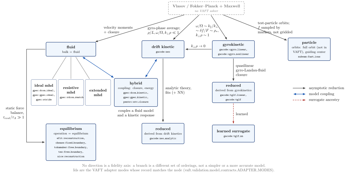
vaft.diagram.plasma_model_reduction_map: every reduction from one kinetic starting point, arrows typed as in the table below; the mode ids under each node are read from the registry.
Arrow labels name the approximation, not “faster” or “more approximate”. Arrows on this page have four meanings, and a diagram must not mix them:
| arrow | meaning | example |
|---|---|---|
| asymptotic reduction | an ordering removes a scale or a variable | Vlasov → drift kinetics by gyro-averaging at $\rho/L\ll1$ |
| model coupling | one model supplies a term to another at run time | δW_k from a drift-kinetic response added to ideal MHD |
| software dependency | one program calls or reads another | GPEC reads DCON’s euler.bin |
| surrogate ancestry | a model is trained on another model’s outputs and stands in for it | TGLF-NN trained on TGLF fluxes |
2. The axes are independent
A model is a point in several independent axes, not a node of one tree. The record keeps them as separate fields
(audit §1, §10, §11). Generated from vaft.code.formalism:
| axis | field | controlled values |
| — | — | — |
| what is computed | scientific_operation | equilibrium, ideal_stability, resistive_stability, perturbed_equilibrium, toroidal_torque, neoclassical_transport, microstability, turbulent_transport, orbit_following, fast_ion_sources |
| bulk description | bulk_description | fluid, hybrid, kinetic, particle, reduced |
| fluid model | fluid_model | ideal_mhd, resistive_mhd, extended_mhd |
| kinetic equation | kinetic_equation | drift_kinetic, gyrokinetic, fokker_planck |
| kinetic coupling | kinetic_coupling | energy, pressure, current, closure, sources |
| distribution formulation | distribution_formulation | delta_f, full_f |
| orbit representation | orbit_representation | full_orbit, guiding_center, gyrocenter, bounce_averaged |
| spatial domain | spatial_domain | local, radially_global, whole_volume |
| topology domain | topology_domain | closed_flux_surface, open_field_line, across_separatrix |
| regime | regime | static, linear, nonlinear, quasilinear, steady_state, time_dependent |
| field model | field_model | mhd_displacement, electrostatic, electromagnetic, prescribed |
Why the words combine freely. “Global δf gyrokinetic PIC” names four independent choices: a radially global
spatial_domain, the delta_f distribution_formulation, the gyrokinetic kinetic_equation, and a
particle-in-cell numerical method (ORB5 is such a code; audit §9). None of the four implies another. Likewise
“local”, “linear” and “electrostatic” are three axes of one CGYRO run, not three levels of approximation.
Numerical representation is not physics. Continuum (Eulerian grid), particle-in-cell, Monte Carlo markers,
finite elements and spectral or shooting methods are ways to solve a model. The record keeps them out of the
common axes and in extensions (audit §11), because the same equation can be solved either way:
| governing model | numerical realization | example |
|---|---|---|
| gyrokinetic | continuum | CGYRO (in VAFT), GENE |
| gyrokinetic | particle-in-cell | ORB5, GTC |
| test-particle Fokker–Planck, guiding centre | Monte Carlo markers | NUBEAM (in VAFT), ASCOT5 |
| linear ideal MHD energy principle | Euler–Lagrange ODE integration in a Fourier poloidal basis | DCON (in VAFT) |
| extended / resistive MHD | finite elements | NIMROD, M3D-C1 |
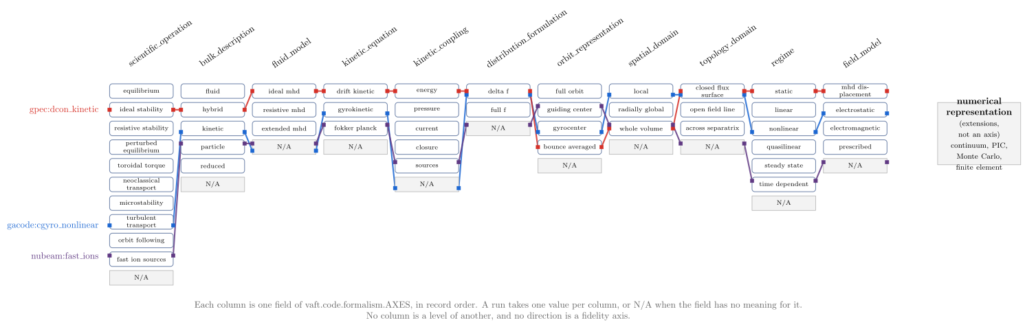
vaft.diagram.formalism_axes_map: one column per axis; three runs (CGYRO nonlinear, DCON kinetic, NUBEAM) drawn across them, so no column is a level of another. Numerical representation sits apart, in extensions.
3. Fluid models
A fluid model evolves velocity moments (density, momentum, pressure) and must close the moment hierarchy. The fluid models differ in which terms of the generalized Ohm’s law and the pressure tensor they keep [2, 3]:
\[\mathbf E + \mathbf v\times\mathbf B = \underbrace{\eta\mathbf J}_{\text{resistive}} + \underbrace{\frac{\mathbf J\times\mathbf B}{ne}}_{\text{Hall}} - \underbrace{\frac{\nabla p_e}{ne}}_{\text{electron pressure}} + \underbrace{\frac{m_e}{ne^2}\frac{d\mathbf J}{dt}}_{\text{electron inertia}}\]Ideal MHD [3] is the momentum equation, the ideal induction equation and an adiabatic pressure law,
\[\rho\frac{d\mathbf v}{dt} = \mathbf J\times\mathbf B - \nabla p,\qquad \frac{\partial\mathbf B}{\partial t} = \nabla\times(\mathbf v\times\mathbf B),\qquad \frac{d}{dt}\left(p\rho^{-\gamma}\right) = 0,\]with $\mu_0\mathbf J=\nabla\times\mathbf B$. Resistive MHD adds $\eta\nabla^2\mathbf B/\mu_0$ to the induction equation (for uniform $\eta$); the other fluid models change Ohm’s law and the closure:
| model | Ohm’s law keeps | pressure closure | fluid_model |
|---|---|---|---|
| ideal MHD | $\mathbf E+\mathbf v\times\mathbf B=0$ | scalar, adiabatic | ideal_mhd |
| resistive MHD | $+\,\eta\mathbf J$ (matters in thin layers at rational surfaces) | scalar | resistive_mhd |
| Hall / two-fluid / extended MHD | $+$ Hall, $\nabla p_e$, electron inertia; separate ion and electron momentum | gyroviscous (FLR), anisotropic, heat-flux closures | extended_mhd |
Reduced MHD is an ordering, not a fourth fluid model. It expands any of these in $\epsilon=a/R$, $\beta$ and
$k_\parallel/k_\perp$ [4]; low aspect ratio weakens its premise. The fluid axis is not the same axis as drift- or
gyrokinetics: a fluid model has no kinetic equation (kinetic_equation=None), and adding Hall or FLR terms does
not make it kinetic (audit §2.1).
Equilibrium is a static fluid problem, $\mathbf J\times\mathbf B=\nabla p$, with the ordering that force balance is restored faster than the state moves ($\tau_{evol}/\tau_A\gg1$). EFIT, CHEASE, TokaMaker, TES and NICE are all this one model (audit §12; NICE provisionally, as an experimental adapter); a kinetic-profile pressure constraint changes their inputs, not their physics.
4. Kinetic models
4.1 Trajectories are not distributions
Two different things are often both called “guiding centre”:
single particle (trajectory variables of ONE particle)       distribution function (a density in phase space)
    |                                                            |
    +-- full orbit:      m dv/dt = q(E + v x B)                  +-- drift kinetic:  f(R, E, mu, t)
    |                                                            |
    +-- guiding-centre orbit: dR/dt = v_par b + v_E              +-- gyrokinetic:    h(R, E, mu, t), finite k_perp rho
                              + v_gradB + v_curv,  mu conserved
Guiding-centre theory [5] reduces the equations of motion of a particle. Drift kinetics evolves a distribution function over the reduced phase space $(\mathbf R, \mathcal E, \mu)$:
\[\frac{\partial f}{\partial t} + \left(v_\parallel\mathbf b + \mathbf v_d\right)\cdot\nabla f + \dot{\mathcal E}\,\frac{\partial f}{\partial\mathcal E} = C(f).\]An orbit integrator alone (SIMPLE) evolves no distribution and is not a drift-kinetic solver. A Monte Carlo code that follows markers with collision kicks (NUBEAM with guiding centres; ASCOT5 with full or guiding-centre orbits) solves a test-particle Fokker–Planck equation by sampling; it is still a statement about a test population in a fixed background, not about the bulk plasma (audit §2.4, §5).
4.2 Drift kinetics and gyrokinetics
Both remove the gyro-phase. They differ in what they keep.
| drift kinetic | gyrokinetic | |
|---|---|---|
| shared | $\omega/\Omega_c\ll1$; gyro-phase averaged; $\rho/L\ll1$ for the background | the same |
| perpendicular scale | long wavelength, $k_\perp\rho\ll1$ | $k_\perp\rho\sim O(1)$ kept, by gyro-averaging the fields |
| what is ordered small instead | — | $\omega/\Omega_i\sim k_\parallel/k_\perp\sim\delta f/F\sim\rho_*$ |
| dynamics kept | guiding-centre drifts, parallel streaming, trapped and passing orbits, bounce resonances | gyro-averaged fluctuating fields acting on gyrocentres |
| typical use | neoclassical transport (NEO), NTV and kinetic stabilization (PENTRC, DCON kinetic) | microinstability and turbulence (CGYRO) |
kinetic_equation |
drift_kinetic |
gyrokinetic |
The gyrokinetic equation in its electrostatic δf form [6] reads, schematically, for the non-adiabatic part $h$ of $\delta f = -q\phi F_0/T + h$:
\[\frac{\partial h}{\partial t} + \left(v_\parallel\mathbf b + \mathbf v_d + \langle\mathbf v_E\rangle_{\mathbf R}\right)\cdot\nabla h - C(h) = \frac{qF_0}{T}\frac{\partial\langle\phi\rangle_{\mathbf R}}{\partial t} - \langle\mathbf v_E\rangle_{\mathbf R}\cdot\nabla F_0 .\]The gyro-average $\langle\cdot\rangle_{\mathbf R}$ is what keeps finite $k_\perp\rho$. At $k_\perp\rho\to0$ it reduces to a drift-kinetic form. So drift kinetics is not a coarse gyrokinetics and gyrokinetics is not an accurate drift kinetics: each keeps physics the other orders out. Neoclassical drift kinetics is also δf, but its $f_1$ is a steady axisymmetric departure, not a fluctuation (audit §2.2–§2.3). The details of which kind of gyrokinetic formulation a run uses (field model, geometry, species, collision operator) belong to #1353.
5. Kinetic-MHD is a coupling, not an equation
A hybrid model keeps a fluid bulk and lets a kinetic population supply part of the force:
          fluid / MHD bulk  (ideal MHD displacement xi, fields)
                |
                |  displacement / perturbed fields
                v
        kinetic population  (drift-kinetic or gyrokinetic response)
                |
                |  pressure tensor / current / energy delta W_k / closure
                v
          fluid / MHD bulk
“Kinetic-MHD” is a family [7]: the population (thermal ions, electrons, energetic particles), the kinetic
equation (drift kinetic, gyrokinetic), the coupling (kinetic_coupling: energy, pressure, current,
closure) and the orbit treatment all vary inside it (audit §2.5). VAFT’s hybrid modes are all in the GPEC suite;
the table shows them with the fluid modes around them. Their record values and contract roles are the generated
rows of §9.
| mode | what it is | hybrid? |
|---|---|---|
gpec:dcon_ideal |
ideal-MHD energy principle | no |
gpec:dcon_kinetic |
ideal MHD + drift-kinetic δW_k added to the Euler–Lagrange coefficients, self-consistent; calling it “drift-kinetic MHD” is provisional (audit §8) | yes, energy coupling |
gpec:gpec_ideal |
ideal-MHD perturbed equilibrium | no |
gpec:gpec_kinetic |
perturbed equilibrium; kinetic content inherited from the DCON run it reads | yes, inherited |
pentrc:ntv_closure |
drift-kinetic closure evaluated on a given displacement; not self-consistent | yes, closure |
gpec:rdcon_rmatch |
outer ideal MHD matched to inner resistive layers | no |
Why RDCON with $T_e$ and $n_e$ is not kinetic-MHD. VAFT passes $T_e$, $n_e$, $Z_{\rm eff}$ and $\ln\Lambda$ to RDCON only to compute the Spitzer resistivity and mass density of each layer (audit §3.4). No kinetic equation is solved. Kinetic profiles as input never make a model kinetic (§8 below).
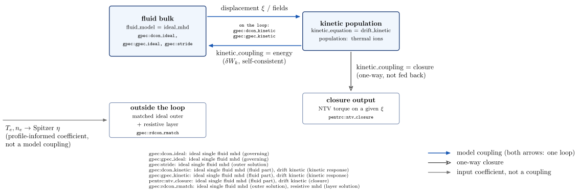
vaft.diagram.kinetic_mhd_coupling: the GPEC-suite modes on the fluid–kinetic loop with their contract roles; RDCON stays outside, with a profile-informed coefficient, not a coupling.
6. Reduced models and surrogates
A reduced model keeps the parent theory of what it approximates, adds a model reduction, and may then be realized by a computational surrogate. These are three separate facts:
| parent theory | model reduction | computational realization | VAFT mode |
|---|---|---|---|
| gyrokinetics | linear eigenmodes of a gyro-Landau-fluid moment system [8] + saturation rule (SAT0–3) → quasilinear fluxes | TGLF | gacode:tglf_linear, gacode:tglf |
| gyrokinetics (through TGLF) | as TGLF, for the SAT variant it was trained on | neural-network surrogate, valid only in its training domain | gacode:tglf_nn |
| drift kinetics | asymptotic reductions of drift-kinetic neoclassical theory reported in a NEO run’s theory output: Hinton–Hazeltine asymptotics, Sauter fits to drift-kinetic solutions, NCLASS moment solutions | closed-form or moment formulas (an asymptotic reduction, not a surrogate) | gacode:neo_analytic |
The record writes this as bulk_description="reduced" with derived_from set to the parent kinetic equation. A
reduced model inherits the orderings of its parent (role inherited in the contract map) and adds a closure
or a fit that no ordering contract covers; the advisory check reports that as unmapped, never as a pass.
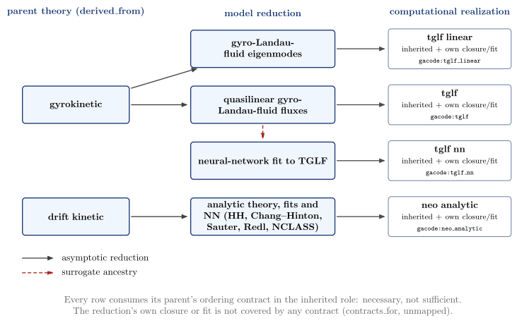
vaft.diagram.reduced_model_ancestry: parent theory, model reduction and computational realization of every reduced mode.
7. What each family is for
Each family is designed for a type of question. This is not a recommendation engine and carries no thresholds: whether a model applies to a given state is an ordering question, answered per state by the contracts of Asymptotic orderings.
| family | designed for | representative assumptions | typically missing |
|---|---|---|---|
| ideal MHD | macroscopic ideal stability and response | $S\gg1$, $\rho/L\ll1$, $\omega\ll\Omega_i$, scales $\gg d_i$, scalar pressure | resistive layers, FLR, kinetic resonances |
| resistive MHD | tearing, reconnection, resistive layers | as ideal MHD outside thin layers; Spitzer η inside | two-fluid and kinetic layer physics when $d_i$ or $\rho_s$ exceeds the layer width |
| drift kinetic | neoclassical transport, orbit-averaged response, NTV | $\omega/\Omega\ll1$, $\rho/L\ll1$, $k_\perp\rho\ll1$ | finite-$k_\perp\rho$ fluctuations, turbulence |
| gyrokinetic | low-frequency microinstability and turbulence | $\omega/\Omega_i\sim k_\parallel/k_\perp\sim\delta f/F\sim\rho_*$ | equilibrium evolution, macroscopic MHD (in a local δf run) |
| particle orbit | confinement, losses, fast-ion slowing down and sources | $\rho/L_B$ small for guiding centre; fixed fields and background | feedback of the particles on fields and bulk |
| hybrid kinetic-MHD | macroscopic modes modified by a kinetic population | the fluid ordering for the bulk plus the kinetic ordering for the population | whatever the coupling leaves out (e.g. finite orbit width, which PENTRC appears not to keep: inferred, not stated in its source) |
The scales these orderings compare, and why a model can hold on one scale and fail on another, are the Characteristic scales and orderings reference (#1724, PR #1985).
Time scales
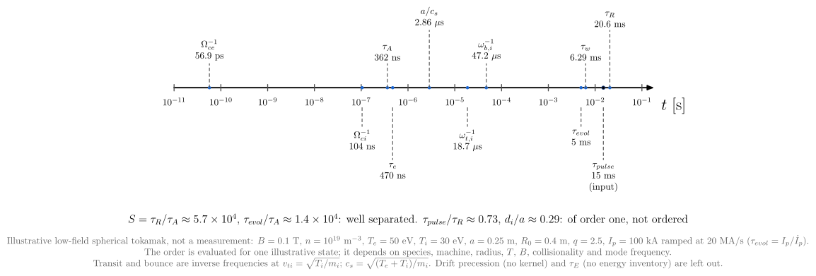
The families above separate along these time scales, written from fast to slow as a class:
gyration 1/Omega_c  ->  bounce / transit 1/omega_b, 1/omega_t  ->  drift precession 1/omega_D  ->  Alfven tau_A
->  sound tau_s  ->  collision tau_c  ->  resistive diffusion tau_R  ->  transport, equilibrium evolution tau_evol
This is not a universal numerical order. The actual order depends on the species, the machine, the radius,
$T$, $B$, the collisionality and the mode frequency; the collision time in particular can sit anywhere in the
chain, and in a low-field device the electron transit frequency can reach the ion gyrofrequency. Drift kinetics
needs the dynamics slower than gyration; gyrokinetics also slower than gyration, but with fluctuations on the
drift scale; MHD needs it slower than the kinetic times its closure averages over; an equilibrium needs
$\tau_{evol}\gg\tau_A$. vaft.diagram.timescale_hierarchy evaluates these times for one labelled illustrative
state (ILLUSTRATIVE_STATE; its assumed values are listed in the figure caption) and places them by value. Drift
precession has no formula kernel and $\tau_E$ needs an energy inventory the state does not carry, so the figure
omits both and says so (#1724).
Spatial scales
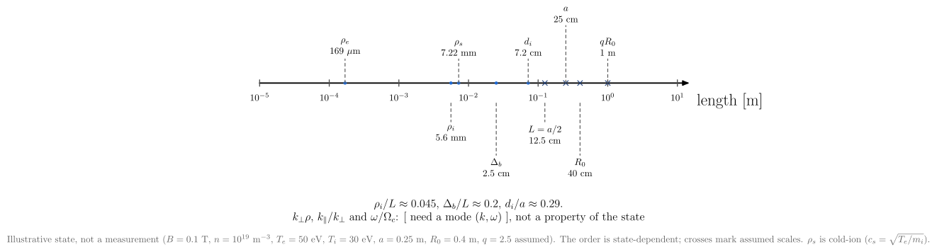
vaft.diagram.spatial_scale_orderings: the lengths of one labelled illustrative state on a log axis, with the ratios the orderings compare; the order is state-dependent.
8. “Kinetic” means seven different things
The same word names a datum, a profile container, a reconstruction constraint, a profile-informed coefficient, a hybrid model, a governing equation and a fitted model. Only the last three describe physics:
| meaning | VAFT example | describes physics? | bulk_description of the model run |
|
|---|---|---|---|---|
| A | measurement or data | “kinetic diagnostics” (Thomson, CES) | no | — |
| B | profile container | KineticProfiles, GPEC/PENTRC kinetic_file |
no | — |
| C | kinetically constrained reconstruction | run_kinetic_efit (EFIT with a pressure constraint) |
no | fluid |
| D | profile-informed coefficient or closure | RDCON’s $T_e$, $n_e$ → Spitzer η; CHEASE closure="kinetic_pressure" |
no | fluid |
| E | hybrid fluid–kinetic model | DCON kin_flag=t, PENTRC |
yes | hybrid |
| F | kinetic governing equation | NEO, CGYRO | yes | kinetic |
| G | derived from kinetic theory | TGLF, Sauter fits | yes | reduced |
The full list of names in each category, and the seven names most likely to mislead, is audit §6. Kinetic-profile input never implies a kinetic governing equation.
9. Every VAFT mode, placed
Generated from vaft.validation.model_contracts.ADAPTER_MODES: one row per scientifically distinct mode, not per
executable. “Contracts (role)” are the ordering contracts the mode consumes, which the advisory ordering check
evaluates on a run’s input (#1823; wiring per stage is #1987); “not covered” is what no contract checks.
Confidence of the rows (audit §3–§5, §12): verified for the equation class of every classified row, except
nice:reconstruction and tglf_nn (provisional, as their audit cell says) and the name “drift-kinetic MHD”
for the DCON and GPEC kinetic modes (provisional). nubeam:fast_ions records guiding_center as its dominant
orbit representation; its FLR position sampling sits in extensions and fits neither orbit value (§10).
| mode | operation | bulk | fluid model | kinetic equation | coupling | orbit | domain | regime | contracts (role) | not covered | audit |
| — | — | — | — | — | — | — | — | — | — | — | — |
| efit:reconstruction | equilibrium | fluid | ideal_mhd | — | — | — | whole_volume | static | quasi_static_equilibrium (governing) | — | Plasma_models.md §12 |
| chease:fixed_boundary | equilibrium | fluid | ideal_mhd | — | — | — | whole_volume | static | quasi_static_equilibrium (governing) | — | Plasma_models.md §12 |
| tokamaker:free_boundary | equilibrium | fluid | ideal_mhd | — | — | — | whole_volume | static | quasi_static_equilibrium (governing) | — | Plasma_models.md §12 |
| tes:free_boundary | equilibrium | fluid | ideal_mhd | — | — | — | whole_volume | static | quasi_static_equilibrium (governing) | — | Plasma_models.md §12 |
| nice:reconstruction | equilibrium | fluid | ideal_mhd | — | — | — | whole_volume | static | quasi_static_equilibrium (governing) | — | Plasma_models.md §12 |
| gpec:dcon_ideal | ideal_stability | fluid | ideal_mhd | — | — | — | whole_volume | static | ideal_single_fluid_mhd (governing) | — | Plasma_models.md §3.1 |
| gpec:dcon_kinetic | ideal_stability | hybrid | ideal_mhd | drift_kinetic | energy | bounce_averaged | whole_volume | static | ideal_single_fluid_mhd (fluid_part), drift_kinetic (kinetic_response) | — | Plasma_models.md §3.2 |
| gpec:gpec_ideal | perturbed_equilibrium | fluid | ideal_mhd | — | — | — | whole_volume | static | ideal_single_fluid_mhd (governing) | — | Plasma_models.md §3 |
| gpec:gpec_kinetic | perturbed_equilibrium | hybrid | ideal_mhd | drift_kinetic | energy | bounce_averaged | whole_volume | static | ideal_single_fluid_mhd (fluid_part), drift_kinetic (kinetic_response) | — | Plasma_models.md §3.3 |
| gpec:rdcon_rmatch | resistive_stability | fluid | resistive_mhd | — | — | — | whole_volume | linear | ideal_single_fluid_mhd (outer_solution), resistive_mhd (layer_solution) | — | Plasma_models.md §3.4 |
| gpec:stride | resistive_stability | fluid | ideal_mhd | — | — | — | whole_volume | linear | ideal_single_fluid_mhd (outer_solution) | — | Plasma_models.md §3.4 |
| gpec:thresholds | unclassified | — | — | — | — | — | — | — | — | the singthresh_* layer models (SLAYER, Callen) are auxiliary reduced layer models whose classification is unresolved in the audit | Plasma_models.md §3 (provisional) |
| pentrc:ntv_closure | toroidal_torque | hybrid | ideal_mhd | drift_kinetic | closure | bounce_averaged | whole_volume | static | ideal_single_fluid_mhd (fluid_part), drift_kinetic (closure) | — | Plasma_models.md §3.5 |
| gacode:neo | neoclassical_transport | kinetic | — | drift_kinetic | — | — | local | steady_state | drift_kinetic (governing), local_neoclassical (governing) | — | Plasma_models.md §4 |
| gacode:neo_analytic | neoclassical_transport | reduced | — | — | — | — | local | steady_state | drift_kinetic (inherited), local_neoclassical (inherited) | a reduced model adds its own closure or fit, which no ordering contract covers | Plasma_models.md §4 (Hinton-Hazeltine, Sauter values in a NEO run’s theory output) |
| gacode:cgyro_linear | microstability | kinetic | — | gyrokinetic | — | gyrocenter | local | linear | gyrokinetic_delta_f (governing) | — | Plasma_models.md §4 (cgyro.plasma_formalism) |
| gacode:cgyro_nonlinear | turbulent_transport | kinetic | — | gyrokinetic | — | gyrocenter | local | nonlinear | gyrokinetic_delta_f (governing) | — | Plasma_models.md §4 (cgyro.plasma_formalism) |
| gacode:tglf_linear | microstability | reduced | — | — | — | — | local | linear | gyrokinetic_delta_f (inherited) | a reduced model adds its own closure or fit, which no ordering contract covers | Plasma_models.md §4 |
| gacode:tglf | turbulent_transport | reduced | — | — | — | — | local | quasilinear | gyrokinetic_delta_f (inherited) | a reduced model adds its own closure or fit, which no ordering contract covers | Plasma_models.md §4 |
| gacode:tglf_nn | turbulent_transport | reduced | — | — | — | — | local | quasilinear | gyrokinetic_delta_f (inherited) | a reduced model adds its own closure or fit, which no ordering contract covers | Plasma_models.md §4 (provisional; a learned surrogate, valid only in its training domain) |
| nubeam:fast_ions | fast_ion_sources | particle | — | fokker_planck | sources | guiding_center | whole_volume | time_dependent | — | test-particle orbit orderings (rho/L_B, slowing down on a fixed background) are not a registered contract | Plasma_models.md §5 |
| genray:ray_tracing | unclassified | — | — | — | — | — | — | — | — | ray tracing (WKB) is neither a fluid nor a kinetic bulk description in the vocabulary | not audited |
| transp:integrated | unclassified | — | — | — | — | — | — | — | — | an integrated-modelling run combines several formalisms; its components are classified | not audited |
| flare:field_lines | unclassified | — | — | — | — | — | — | — | — | field-line tracing through a given equilibrium and 3-D perturbation: magnetic topology only, no plasma model is solved, so no plasma formalism applies | vaft/code/flare.py |
| mitim:drivers | unclassified | — | — | — | — | — | — | — | — | a driver: the NEO and TGLF runs it launches are the gacode:neo and gacode:tglf modes; PORTALS flux matching (#1588, not yet in VAFT) will be transport_coupled | vaft/code/mitim (#1588) |
Not in VAFT. These codes are classified for comparison and interoperability only. The ASCOT5 row is verified from upstream documentation (audit §5); the others are provisional, from literature (audit §5, §9). None has a VAFT run adapter; ASCOT5 appears only as a diagram catalogue entry.
| code | bulk | kinetic equation / fluid model | domain | numerical realization | | — | — | — | — | — | | GENE / GENE-X | kinetic | gyrokinetic; GENE-X full-f, across the separatrix | local or global; GENE-X whole volume | continuum | | GTC | kinetic | gyrokinetic ions and energetic particles (GTC-X: no primary reference identified) | global | PIC | | ORB5 | kinetic | gyrokinetic, δf with control variates | global | PIC | | MARS-F / MARS-K | fluid / hybrid | resistive MHD with flow and wall; MARS-K adds drift-kinetic resonances | whole volume | — | | ASCOT5 | particle | test-particle Fokker–Planck | whole volume | Monte Carlo, full or guiding-centre orbit | | SIMPLE | particle | none (orbit integration) | whole volume | symplectic guiding-centre integrator |
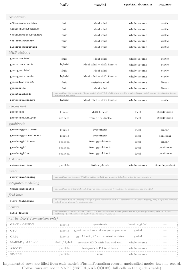
vaft.diagram.solver_placement_map: every registered mode against the axes of §2; codes not in VAFT (vaft.diagram.EXTERNAL_CODES) are hollow.
10. Still unresolved
These classifications are open and are shown as such, not smoothed over (audit §8):
- No record: the GPEC threshold layer models (
gpec:thresholds; SLAYER, Callen), GENRAY ray tracing (WKB is neither a fluid nor a kinetic bulk description), TRANSP integrated runs (combinations of formalisms), FLARE field-line tracing (topology only, no plasma model) and the MITIM drivers (the NEO and TGLF runs they launch carry their own records). They are listed in the matrix as unclassified with the reason. - No contract: NUBEAM’s test-particle orbit orderings ($\rho/L_B$, slowing down on a fixed background) are not a registered ordering contract, and a reduced model’s own closure or fit is covered by none.
- DCON and GPEC (evidence missing):
- whether DCON kinetic is “drift-kinetic MHD” in the sense of Park (2011) and Park & Logan (2017);
- the Kruskal–Oberman correspondence (PENTRC implements a CGL limit; no KO-labelled limit exists in its source);
- how the fluid compressional term and δW_k are partitioned (possible double counting);
- finite orbit width in PENTRC (inferred absent, not stated);
- the derivation of the “harmonic” collision model;
- the physics of the SLAYER and Callen threshold models.
- GACODE (evidence missing): the class of CGYRO’s collision operator, and whether NEO’s and CGYRO’s operators share a category; the FLR content of TGLF’s moments; the training provenance of the TGLF-NN models VAFT resolves.
- Taxonomy design: NUBEAM’s guiding centre + FLR sampling fits neither orbit value; whether full orbit belongs under the kinetic equation or the orbit representation (the record puts it under orbit representation); pressure versus current coupling in hybrid codes (MEGA, MARS-K); how kinetic reduced MHD (KRMHD) is represented.
- Pending backend adoption: the GACODE records still trust parts of the run configuration (#1735).
11. Glossary
Where a term has a controlled value in vaft.code.formalism, the value is given; the test checks that every value
named here exists. A term without one is not part of the record, on purpose.
| term | meaning | record value |
| — | — | — |
| MHD | single-fluid magnetohydrodynamics; ideal (no dissipation) or resistive | fluid_model: ideal_mhd, resistive_mhd |
| extended MHD | fluid closures beyond resistive MHD: Hall, electron pressure and inertia, gyroviscosity, anisotropic pressure | fluid_model: extended_mhd |
| kinetic MHD | a fluid bulk with a kinetic response of selected populations; a family of couplings | bulk_description: hybrid |
| hybrid | any fluid–kinetic coupled description | bulk_description: hybrid |
| closure | the relation that ends a moment hierarchy; in the record, a kinetic result evaluated on a given fluid displacement | kinetic_coupling: closure |
| Vlasov / Fokker–Planck | the full kinetic equation, collisionless or collisional; no VAFT solver evolves it for the bulk plasma | none for the bulk |
| test-particle Fokker–Planck | the kinetic equation of a test population in a fixed background, as NUBEAM solves it | kinetic_equation: fokker_planck |
| guiding centre | the gyro-averaged position of a particle and its drift equations of motion | orbit_representation: guiding_center |
| full orbit | the particle trajectory under the full Lorentz force | orbit_representation: full_orbit |
| drift kinetic | a kinetic equation for the gyro-averaged distribution at $k_\perp\rho\ll1$ | kinetic_equation: drift_kinetic |
| gyrokinetic | a kinetic equation for the gyrocentre distribution keeping $k_\perp\rho\sim1$ | kinetic_equation: gyrokinetic; orbit_representation: gyrocenter |
| FLR | finite-Larmor-radius effects: corrections in $k_\perp\rho$ or $\rho/L$ | none (solver detail) |
| δf | the distribution split into a known background and a small perturbation that is evolved | distribution_formulation: delta_f |
| full-f | the whole distribution is evolved | distribution_formulation: full_f |
| local | a flux tube or a single surface, with profiles and gradients taken at one radius | spatial_domain: local |
| global | a radial range with profile variation, or the whole plasma volume | spatial_domain: radially_global, whole_volume |
| continuum | a solution on a phase-space grid (Eulerian) | none (extensions) |
| PIC | particle-in-cell: markers sample the distribution; fields on a grid | none (extensions) |
| Monte Carlo | stochastic markers, e.g. for collisions in a test-particle Fokker–Planck solution | none (extensions) |
| surrogate | a model trained on another model’s outputs to stand in for it (an analytic fit to a theory is a reduction, not a surrogate) | bulk_description: reduced; derived_from: gyrokinetic |
References
- P. Helander and D. J. Sigmar, Collisional Transport in Magnetized Plasmas, Cambridge University Press (2002).
- S. I. Braginskii, in Reviews of Plasma Physics, Vol. 1, Consultants Bureau (1965), p. 205.
- J. P. Freidberg, Ideal MHD, Cambridge University Press (2014).
- H. R. Strauss, Phys. Fluids 19 (1976) 134.
- R. G. Littlejohn, J. Plasma Phys. 29 (1983) 111; J. R. Cary and A. J. Brizard, Rev. Mod. Phys. 81 (2009) 693.
- E. A. Frieman and L. Chen, Phys. Fluids 25 (1982) 502; A. J. Brizard and T. S. Hahm, Rev. Mod. Phys. 79 (2007) 421.
- M. D. Kruskal and C. R. Oberman, Phys. Fluids 1 (1958) 275; C. Z. Cheng, Phys. Rep. 211 (1992) 1.
- G. M. Staebler, J. E. Kinsey and R. E. Waltz, Phys. Plasmas 14 (2007) 055909; G. W. Hammett and F. W. Perkins, Phys. Rev. Lett. 64 (1990) 3019.
Primary sources for each backend mode (upstream source lines, solver papers) are in the audit page.