Plasma parameter inference
Plasma parameter inference determines a plasma-state quantity that no diagnostic measured, from quantities VAFT already has, together with explicit physical constraints, closures and assumptions:
known plasma state + physical closure + explicit prior / assumption -> missing plasma parameter
It sits between two neighbours and is neither of them:
- Profile reconstruction turns measurements into a profile through a measurement model and a fit
(
measurements -> fit -> profile). Multi-diagnostic fitting of one primitive profile (TS + interferometer, TS + ECE, CX + other diagnostics) stays there — see Equilibrium and kinetic profiles and #1204. The fit carries its own assumptions — the basis (polynomial, core-polynomial/edge-exponential, Gaussian process) and its order, the fitting coordinate ($\rho_{\mathrm{tor},N}$ or $\psi_N$), positivity and uncertainty weighting — and the overview draws them entering the reconstructed profiles, because every closure below inherits them. - Simulation and consistency workflows take a completed state into NEO, TGLF, CGYRO, CHEASE and predict a response or test consistency. A flux-matched profile may come out of an inverse solve, but it is transport-model-consistent, not a closure-inferred experimental parameter. The equilibrium–kinetic iteration (#123) belongs there too.
The principle throughout: VAFT may complete an incomplete plasma state through explicit physical
constraints, but every inferred or synthetic quantity stays distinguishable from a measurement and
traceable to the assumptions and inputs that produced it. This page documents the pathways that exist
on develop; it introduces no new computational layer and no Inference runtime object.
How a quantity was obtained
| Origin | Meaning | VAFT example |
|---|---|---|
| measured | a diagnostic determined it | Thomson T_e, n_e; CX T_i |
| reconstructed | the solution of an inverse problem or fit | EFIT p_eq(ψ); fitted T_e(ρ) |
| inferred | estimated through a stated closure from other data | pressure-partition T_i; resistive Z_eff |
| assumed | supplied by the user or the machine policy | T_i/T_e ratio; a composition preset |
| synthetic | completed from an equilibrium and assumptions, with no kinetic data | core_profiles_from_eq, generate_synthetic_kinetic_profiles |
| predicted | the output of a transport or stability model | TGLF fluxes; flux-matched profiles |
The diagrams use the same grammar as the physics-workflow diagrams (#1585), draw only the closures VAFT implements today, and number each closure’s representative papers; synthetic completion and force balance are described in their sections below.
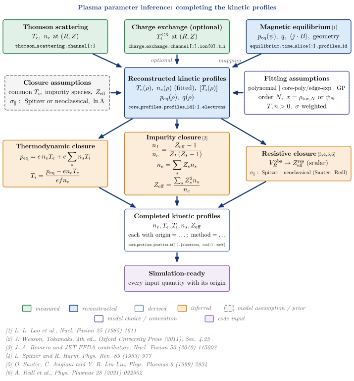
Thermodynamic closure
The thermal pressure is
\[p_{\mathrm{th}} = p_e + p_i = e\,n_e T_e + e \sum_s n_{i,s} T_{i,s}.\]Pressure alone does not determine density and temperature: $p = nT$ is underdetermined until one more constraint is supplied.
p_eq alone                     x->  unique n_e, T_e
p_eq + n_e                      ->  T_e (or T_i)
p_eq + T_e                      ->  n_e
p_eq + one more profile/scalar  ->  a possible kinetic decomposition
Ion temperature from the equilibrium pressure
With an equilibrium pressure, fitted electron profiles and an ion-density closure $\sum_s n_{i,s} = f\,n_e$ (common ion temperature),
\[p_i = p_{\mathrm{eq}} - e\,n_e T_e, \qquad T_i = \frac{p_i}{e\,f\,n_e} = \frac{p_{\mathrm{eq}}}{e f n_e} - \frac{T_e}{f}.\]vaft.process.kinetic_closure.infer_ti_pressure_partition implements this (#1426). It propagates
the uncertainty linearly — keeping the $n_e$ correlation between $p_e$ and the ion density — and
flags points, never fills them: $p_i \le 0$ and $p_i < \sigma(p_i)$ return NaN. It also refuses a
circular input: a pressure reconstructed with an assumed $T_i/T_e$ (a kinetic EFIT) returns that
assumption, so only an independent ("magnetics") equilibrium lineage is eligible. The composition
dependence enters through $f$, which the impurity closure supplies.
Temperature or density from the equilibrium pressure
The two inverse directions — solve $T_e$ given $n_e$, or $n_e$ given $T_e$, each with a declared
$T_i/T_e$ and composition — are closures of generate_synthetic_kinetic_profiles with
pressure_constraint="equilibrium" and closure="temperature" or "density". They make
$p_{\mathrm{kin}} = p_{\mathrm{eq}}$ locally. Because the held channel is itself an assumption when no
kinetic data enter, these results are synthetic (next section) unless the held profile is measured.
Equilibrium-constrained synthetic completion
When there are no kinetic measurements at all, VAFT can still complete a state from the equilibrium,
and labels it synthetic. The simplest closure (core_profiles_from_eq, core_profiles_from_eq_ratio)
assumes $n_e$ and $T_e$ share one shape:
with $k = 2$ for pure hydrogen and $T_i = T_e$ ($p_{\mathrm{eq}} = 2 e n_e T_e$).
generate_synthetic_kinetic_profiles (#122) generalizes it as a fidelity ladder:
| Level | Closure |
|---|---|
| 0 | SqrtPressureSplit — the $\sqrt{p}$ decomposition above, bit for bit |
| 1 | analytic profile shapes (AnalyticProfile) or tabulated shapes |
| 2 | scalar-normalized: axis, separatrix, line or volume average, peaking, Greenwald fraction, $T_i/T_e$ or $p_e/p$ |
| 3 | a prescribed $a/L$ profile |
Every target is recomputed from the final arrays and reported as requested versus achieved; the slice it writes says it is synthetic. This is state completion, not a unique kinetic inference from EFIT. Details: Equilibrium and kinetic profiles.
Impurities and quasineutrality
\[n_e = \sum_s Z_s n_s, \qquad Z_{\mathrm{eff}} = \frac{\sum_s Z_s^2 n_s}{n_e}.\]Once a composition model is declared — the relative impurity weights $w_s$ — these two relations fix the
main-ion density, the impurity densities and the dilution at a target $Z_{\mathrm{eff}}$
(vaft.formula.impurity.solve_impurity_mixture_for_target_zeff). With more species or charge states
than constraints the problem is underdetermined, which is why the weights must be declared.
vaft.process.impurity.resolve_impurity_composition decides which composition applies and records why,
in a fixed order: stored ions labelled measured → an explicit argument → a derived composition
(a stated model) → stored ions labelled assumed or unlabelled → the machine preset. A fixed,
fully stripped impurity closure is this algebra with $Z_s$ constant; atomic charge-state inference
replaces $Z_s$ by the moments $\langle Z\rangle_s = \sum_q q f_{s,q}$ and
$\langle Z^2\rangle_s = \sum_q q^2 f_{s,q}$ (next sections). The provenance it writes on core_profiles
uses one grammar: origin=<measured|assumed|derived|inferred>; method=<m>[; key=value...].
Resistive Z_eff
vaft.process.resistive_zeff infers one scalar effective charge over a time window: the
$Z_{\mathrm{eff}}$ a chosen parallel-conductivity model needs to reproduce the plasma resistance observed
through Romero’s transformer balance.
equilibrium + transformer balance  ->  V_R^obs, R_p^obs
T_e, n_e + conductivity model      ->  R_p^model(Z)
bounded scalar fit                 ->  Z_eff^res,obs
$Z_{\mathrm{eff}}^{\mathrm{res,obs}}$ is model-inferred from global electrical behaviour: it depends on
the conductivity model (Spitzer, Sauter, Redl) and on $\ln\Lambda$, and it is not a composition measurement.
It is never interchangeable with a local composition $Z_{\mathrm{eff}}^{\mathrm{comp}}(\rho)$ —
resolve_impurity_composition carries it beside a composition under its own provenance and never uses
it as a target. See the resistive Z_eff diagram.
Atomic-model-constrained Z_eff(ρ)
On develop since PR #1659 (Lane L / Lane Z: #1565, #1566, #1569):
vaft.process.impurity.resolve_radial_composition(..., normalization="resistive_closure", projection=...,
resistive_target=...)
. The chain combines radial structure from atomic physics with a global amplitude
from the resistive closure:
T_e(ρ), n_e(ρ), plasma age  +  elemental-ratio prior (C/O)
    -> transient charge states f_{s,q}(ρ)  ->  <Z>_s(ρ), <Z²>_s(ρ)
    -> n_C/n_e = a w_C,  n_O/n_e = a w_O  ->  Z_eff(ρ; a)
    -> resistive projection  Z_eff(ρ; a) --P_R--> Z_eff^res,equiv(a)
    -> a*: Z_eff^res,equiv(a*) = Z_eff^res,obs  (bracketed root-find)   ->   Z_eff(ρ; a*)
Atomic physics sets the radial charge-state structure (ionization="coronal" or "transient" with
plasma_age_s); the resistive closure sets one impurity amplitude, the projection callable being the
resistive projection P_R of #1566 and resistive_target the observed resistive Z_eff. The result is
closure-inferred, not a unique composition measurement; populate_radial_impurity_profiles writes it to
core_profiles with <Z>(ρ), <Z²>(ρ) per element.
Rotation and force balance — future scope
No VAFT pathway infers rotation or the radial electric field yet. The relevant quantities are $V_\phi$, $V_\theta$, $\Omega_\phi$, $E_r$ and the ExB shear $\gamma_E$; a representative relation is
\[E_r = \frac{1}{Z_i e n_i}\frac{dp_i}{dr} + V_\phi B_\theta - V_\theta B_\phi\](in the adopted sign convention). One force-balance equation does not determine $E_r$, $V_\phi$ and $V_\theta$ independently; a future inference would combine CXRS rotation, a neoclassical poloidal-flow model, pressure gradients and the equilibrium geometry. The source order should be measured > closure-inferred > model-predicted > explicit zero-rotation assumption.
Today TGLF and CGYRO receive $\gamma_E = 0$ as an explicit assumption (#553). A zero-rotation assumption must never be presented as inferred rotation.
Inferred quantities depend on inferred quantities
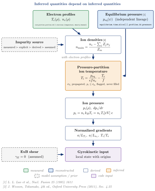
A composition assumption fixes the ion densities, which set the pressure-partition $T_i$, whose gradient would enter force balance and the ExB shear a gyrokinetic input needs. Uncertainty and provenance propagate down this chain, so each inferred profile should answer where did this come from? A record for an inferred quantity names:
quantity, origin, method
depends_on      (input quantities and their origins)
assumptions
validity        (conditions under which the closure holds)
uncertainty / sensitivity
downstream consumers
For example, the pressure-partition result returns
origin="inferred", method="equilibrium_pressure_partition", its equilibrium_lineage, its
assumptions (common ion temperature and the composition source), per-point flags and
$\sigma(T_i)$; a composition written to core_profiles carries origin=...; method=.... There is no
single runtime provenance object, by design.
Worked examples
A — EFIT-only Level-0 state (synthetic)
import vaft

ods = vaft.omas.sample_ods()                    # an ODS holding an equilibrium
vaft.process.core_profiles_from_eq(ods, Te0_eV=100.0, eq_time_index=0)
cp = ods["core_profiles.profiles_1d.0"]
cp["electrons.temperature"][0], cp["electrons.density_thermal"][0]   # 100 eV, ~1.0e18 m^-3
$p_{\mathrm{eq}} \to n_e, T_e, T_i = T_e, n_i = n_e$. The result is synthetic: the on-axis temperature and the shared shape are assumptions, not data.
B — ion temperature from the equilibrium pressure (inferred)
import numpy as np
from vaft.process.kinetic_closure import infer_ti_pressure_partition

result = infer_ti_pressure_partition(
    np.array([500.0, 330.0, 120.0]),              # p_eq [Pa], magnetic-only equilibrium
    np.array([1.2e19, 1.0e19, 0.6e19]),           # n_e [m^-3], fitted
    np.array([150.0, 110.0, 60.0]),               # T_e [eV], fitted
    composition={"ion_density_per_electron": 0.9,
                 "composition_source": "assumed: carbon at Z_eff = 1.5"},
    sigma_p_eq=np.array([50.0, 40.0, 30.0]), sigma_n_e=np.full(3, 1e18),
    sigma_t_e=np.array([10.0, 10.0, 8.0]),
    equilibrium_lineage="magnetics",
)
result["t_i"], result["sigma_t_i"]                # ~[122, 107, 72] eV, ~[39, 38, 43] eV
With equilibrium_lineage="kinetic" the call returns eligible=False and the reason: that pressure was
fitted with an assumed $T_i/T_e$, so partitioning it would return the assumption.
C — electron density from the equilibrium pressure (synthetic)
from vaft.data import Composition, ProfileSpec, ScalarTarget, SyntheticKineticSpec, TemperatureAssumption
from vaft.data.resources import sample_geqdsk
from vaft.process.profile import compose_analytic_profile, generate_synthetic_kinetic_profiles

te_shape = compose_analytic_profile("T_e", axis_value=1.0, separatrix_value=0.1, core_beta=2.0)
spec = SyntheticKineticSpec(
    T_e=ProfileSpec(te_shape, ScalarTarget("axis", 150.0)),    # held: an assumed T_e
    temperature=TemperatureAssumption(ti_over_te=0.5),
    composition=Composition("D", "C", z_eff=2.0),
    pressure_constraint="equilibrium", closure="density",      # solve n_e so p_kin = p_eq
)
result = generate_synthetic_kinetic_profiles(sample_geqdsk(), spec, time=0.319)
result.status, [(t.name, t.requested, t.achieved) for t in result.targets]
Every requested target comes back as requested versus achieved. With a fitted $T_e$ in place of the assumed shape, the same closure becomes an inference of $n_e$ from data.
D — resistive Z_eff (inferred)
compute_romero_flux_balance_ods(ods)        ->  V_R^obs(t), R_p^obs(t)
observed_resistance(...)                    ->  observed series on the window
infer_resistive_zeff(observed, states,
    model=..., ln_lambda=..., bounds=..., weights="uniform")   ->  Z_eff^res ± σ, residual, bound hit
The bounds are set by the caller; there is no VAFT default. See vaft.omas.resistive_zeff for the
ODS-level entry point.
E — atomic + resistive Z_eff(ρ)
from vaft.process.impurity import resolve_radial_composition, populate_radial_impurity_profiles

radial = resolve_radial_composition(te, ne, rho, {"C": 1, "O": 1},
                                    normalization="resistive_closure",
                                    projection=P_R, resistive_target=zeff_res_obs)
ods = populate_radial_impurity_profiles(ods, radial)
P_R is the resistive projection Z_eff(ρ) -> scalar (#1566; it receives NaN at undefined points and
must ignore them); see above.
Related
- Equilibrium and kinetic profiles — profile fitting, synthetic profiles, EFIT
- Computational layers — Formula / Process / Code
- Formula reference and Scientific diagrams
- Issues: #1204 (profile evidence), #122 (synthetic profiles), #123 (equilibrium–kinetic iteration), #1426 (pressure-partition T_i), #1565 / #1566 / #1569 (impurity and Z_eff), #553 (rotation inputs)