Gyrokinetic plotting
After a local gyrokinetic or reduced turbulent-transport calculation, a plasma physicist
inspects the same few things: linear growth rates and frequencies, where in $k_y$ the flux
is carried and by which field, the fluctuation amplitudes and cross phases, the mode
structure, and the local plasma state that produced all of it. Then they look at the
fluxes as radial profiles and compare models. This page maps those quantities onto VAFT
(issue #1591). MITIM’s TGLF.plot answers the same questions and is used here as a
benchmark of what is worth showing. MITIM is not imported, and its layout is not copied.
Two families, two layers
| local gyrokinetic | radial turbulent transport | |
|---|---|---|
| scientific object | one flux tube: (shot, time, surface, solver) | fluxes vs $\rho_{tor,N}$ for one time slice |
| IMAS home | gyrokinetics_local (one simulation per IDS) |
core_transport.model[:] (anomalous, index 6) |
| typical views | $\gamma(k_y)$, $\omega(k_y)$, flux spectra, field contributors, eigenfunctions, local state | $Q_e(\rho)$, $Q_i(\rho)$, $\Gamma_s(\rho)$, model-to-model comparison |
The two families are kept separate on purpose. A gyrokinetics_local IDS describes one
local calculation, not a radial collection of them.
Each family has two layers:
- Native (
vaft.plot.gyrokinetics). These are solver diagnostics in GACODE units: $k_y\rho_s$, $\gamma$ and $\omega$ in $c_s/a$, $\omega$ with the ion diamagnetic direction negative. That is TGLF’s own sign. CGYRO’s native sign depends on the field orientation, so it is converted using the ion direction CGYRO reports for each run (CgyroOutputs.frequency_ion_negative). On the #1482 surfaces the two codes agree on the branch at 78 of 82 converged points. Matched TGLF–CGYRO validation uses this layer, because both codes share the normalization. - Standardized. These are registered plots that read the IMAS IDS in its GKDB normalization:
binormal_wavevector_norm,growth_rate_norm, lengths in units of $R_0$, $v_{th,ref}=\sqrt{2T_e/m_D}$.
A native quantity is never fed to a standardized plot, nor the reverse. Conversions live in the mapping layer (vaft.machine_mapping.gyrokinetics.conversion_factors), not in renderers.
Linear, quasilinear and nonlinear coverage
| output | TGLF (quasilinear) | CGYRO linear | CGYRO nonlinear |
|---|---|---|---|
| $\gamma, \omega$ vs $k_y$ | all NMODES per $k_y$ |
one converged eigenvalue per run | — |
| flux spectrum by field | saturated sum_flux_spectrum |
quasilinear weights only | time-averaged ky_flux |
| fluctuation amplitudes, cross phase | model spectra | — | from kxky_* (not yet parsed) |
| eigenfunction | wavefunction (single-$k_y$ run, not parsed) |
ballooning $\phi$, $A_\parallel$ | — |
| validity | preset family (SAT rule couples the linear model) | converged / max-time / decayed | saturation window, locality QA |
TGLF’s presets couple the linear model to the saturation rule. SAT0 runs with XNU_MODEL=2. SAT2/3 switch to XNU_MODEL=3 and WDIA_TRAPPED=1 (tglf_startup.f90). So “TGLF linear” always names its preset family.
UNITS=CGYRO (forced for SAT2/3) only moves where TGLF places the $k_y$ grid (ky_factor = grad_r0). Reported $k_y$ and $\gamma$ keep the same normalization, and spectra from the two families overlay correctly.
Coverage matrix: MITIM benchmark → VAFT
Native source: the parsed field of TglfOutputs / CgyroOutputs. IMAS class follows the mapping audit (MAPPING_AUDIT): exact, unit, coordinate, derived, convention, unsupported.
| MITIM tab | quantity | native source | IMAS home | class | VAFT plot |
|---|---|---|---|---|---|
| Summary | $\gamma(k_y)$, $\omega(k_y)$ | growth_rate, frequency (TGLF, all modes); CGYRO final eigenvalue |
linear.wavevector[:].eigenmode[:].growth_rate_norm / frequency_norm |
unit / convention (CGYRO mapped) | native plot_linear_spectrum; standardized gyrokinetics_spectrum_growth_rate / _frequency |
| Summary | $\gamma/k$ view | derived from the spectrum | — | reduced diagnostic | native plot_mixing_length_proxy (explicit $\gamma/k_y^2$ at $k_x=0$ or $\gamma/k_y$) |
| Summary | $\delta T_e$, $\delta n_e$ amplitudes | temperature_spectrum, density_spectrum |
none audited | unsupported | native plot_fluctuation_spectra |
| Summary | $n_e$–$T_e$ cross phase | nete_crossphase_spectrum |
none audited | unsupported | native plot_fluctuation_spectra |
| Summary | $Q_e, Q_i, \Gamma_e$ spectra | sum_flux_spectrum (TGLF); flux (CGYRO NL) |
non_linear.fluxes_1d per field (totals only) |
unit (CGYRO mapped) | native plot_flux_ky_spectrum, plot_flux_contributors; standardized gyrokinetics_spectrum_energy_flux / _particle_flux (per $k_y$ from fluxes_2d_k_x_sum) |
| Summary / Exp. Fluxes | $Q_e(r), Q_i(r), \Gamma_e(r)$ | gbflux × gyro-Bohm unit |
core_transport.model[:].profiles_1d |
unit (TGLF, CGYRO mapped) | standardized turbulent_transport_profile_energy_flux / _particle_flux |
| Contributors | flux by field ($\phi$, $A_\parallel$, $B_\parallel$) | sum_flux_spectrum[:, field] |
non_linear.fluxes_1d.*_<field> |
unit | native plot_flux_contributors (only fields the solver wrote; no ES/EM by difference) |
| Spectra | intensities per species and mode | intensity_spectrum |
none audited | unsupported | parsed; not drawn yet |
| Fields: $\phi$ / $A_\parallel$ / $B_\parallel$ | field intensity spectra | field_spectrum |
none audited | unsupported | parsed; not drawn yet |
| Fields | QL weights per mode | ql_flux_spectrum |
linear_weights |
unsupported (amplitude normalization) | parsed; never labelled as a flux |
| Model Details | Gaussian width, spectral shift, $\langle p_0\rangle$ | width_spectrum, spectral_shift_spectrum, ave_p0_spectrum |
— | solver-native | native plot_model_details |
| SAT Parameters | SAT scalars, geometry factors | saturation_parameters |
code.parameters |
provenance | native plot_saturation_parameters |
| WF @ ky | eigenfunction | CGYRO ballooning; TGLF wavefunction (not parsed) |
eigenmode[:].fields.*_perturbed_norm |
convention ($\phi$ mapped, $A_\parallel$ native) | native plot_eigenfunction; standardized gyrokinetics_profile_eigenfunction |
| Input Plasma | species gradients, $q$, $s$, $\kappa$, $\beta$, $\nu$ | TGLFInput, CGYROInput |
species[:], flux_surface, species_all |
exact / unit | native plot_local_state (with provenance kinds) |
| Input Controls | solver settings | input.tglf.gen, input.cgyro.gen |
code.parameters |
provenance | not plotted |
| Simple / Fluctuations / Normalization | SI fluxes, synthetic diagnostics | need input.gacode normalization |
— | — | out of first scope |
Comparing solvers
An overlay does not prove that two runs are matched. A comparison is meaningful only when both runs share:
- the plasma state and surface;
- species, geometry and field model;
- normalization and frequency sign convention.
In VAFT, CGYRO’s input is a renaming of the TGLF local input, so a TGLF–CGYRO native comparison satisfies this by construction. The standardized views check the same conditions against each IDS’s own metadata, and they mark a mismatch on the figure instead of overlaying silently.
Example: one VEST state
These figures are built from existing Lane Y products by workflow/gyrokinetic/build_plot_example.py. The state is shot 39915 at 0.317 s (magnetics lineage), and the field model is EM ($A_\parallel$). The registered plots read only the IMAS IDS, never solver files.
import vaft.omas
from vaft.machine_mapping.gyrokinetics import merge_linear_scan

cgyro = merge_linear_scan(single_ky_odss)          # one CGYRO run per k_y -> one IDS
vaft.omas.plot_gyrokinetics_overview(cgyro)
vaft.omas.plot_gyrokinetics_spectrum_growth_rate({"CGYRO": cgyro, "TGLF SAT2": tglf})
vaft.omas.plot_turbulent_transport_overview({f"TGLF SAT{n}": ct for n, ct in sat_rules.items()})
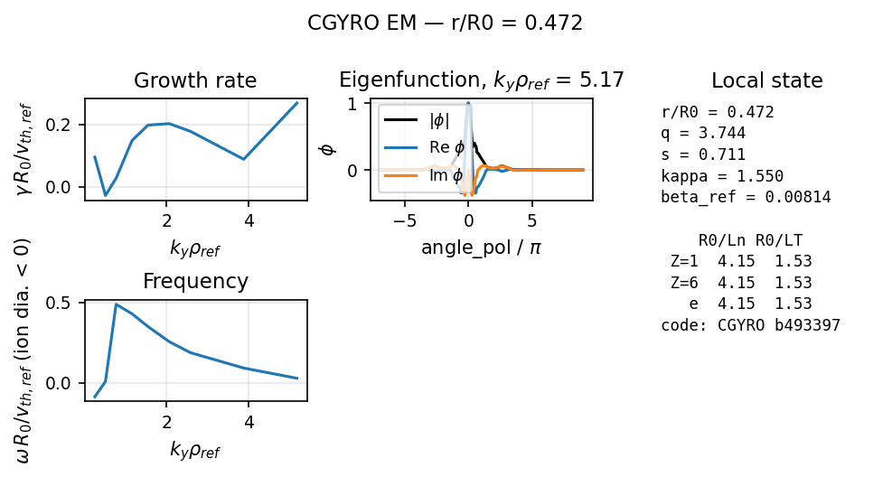
CGYRO overview (r/a 0.7). The 12 linear runs on this surface are merged into one gyrokinetics_local (merge_linear_scan). Merging refuses runs whose species, surface or model differ. Initial-value eigenmodes that stopped at the time limit carry no growth_rate_tolerance, so they are left out. Pass include_unconverged=True to draw them. The eigenfunction panel shows the most unstable converged mode.
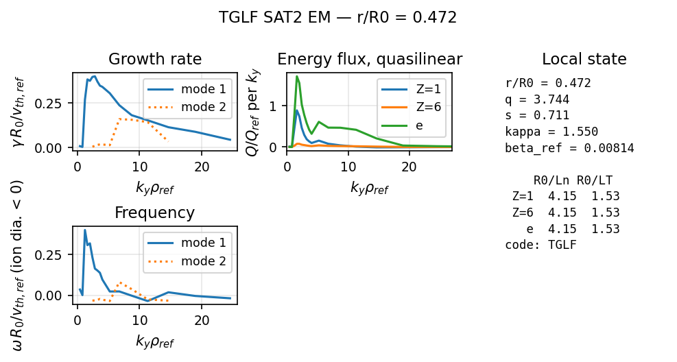
TGLF SAT2 overview, same surface. It is mapped by gyrokinetics_local_from_tglf. TGLF writes every eigenmode (here two) and the quasilinear flux per $k_y$, so the overview gains a flux panel. The $k_y$ axis of that panel stops where every species’ flux has fallen below 1% of its peak. Nothing is dropped from the data.
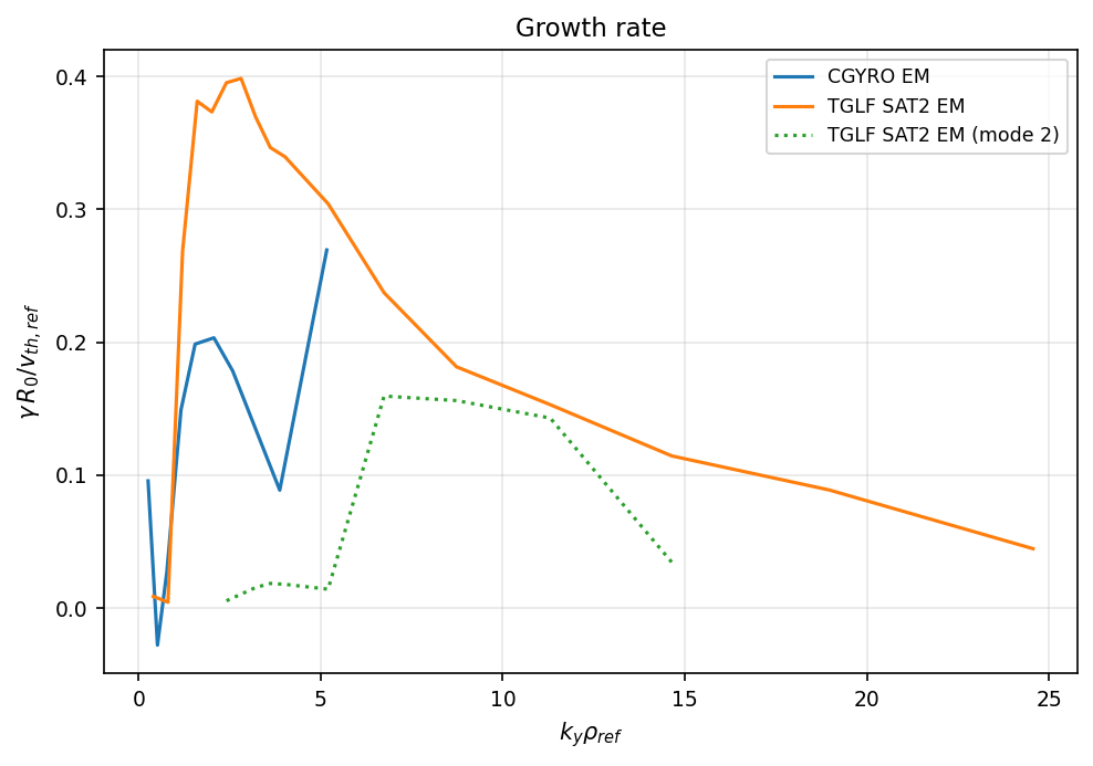
Matched comparison. Both IDS describe the same surface, species, field model, normalization and sign convention, so the overlay carries no “unmatched” note. The TGLF SAT2-preset growth rate lies above CGYRO’s converged points, as in the #1484 validation.
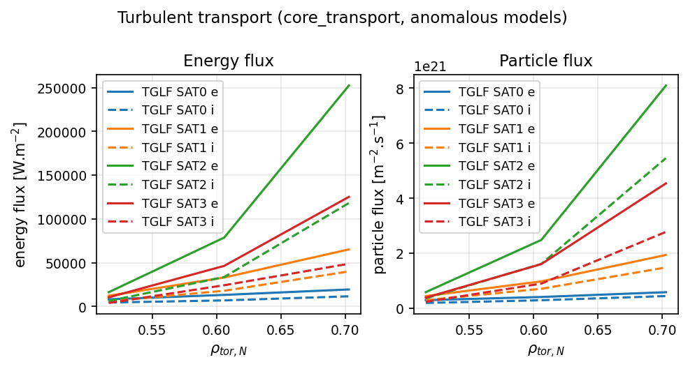
Radial family. core_transport with one anomalous model per SAT rule over r/a 0.6-0.8. Each model gets one color, with electrons solid and ions dashed.
Turbulence–zonal-flow (predator–prey) views
Three native views in vaft.plot.gyrokinetics (#1820) draw what vaft.process.gyrokinetics derived from a nonlinear run. They do not detect peaks, correlate or fit anything themselves.
| view | draws | takes |
|---|---|---|
plot_predator_prey_trace |
$N(t)$, $E(t)$ and optionally $Q(t)$ in stacked panels | the traces, plus an optional PredatorPreyFit (dashed, on its own window) and an optional PredatorPreyCycleMetrics (peak markers) |
plot_predator_prey_phase_space |
the measured $N$–$E$ trajectory, coloured by time and with direction arrows | an optional fit, which adds the fitted orbit, both nullclines ($\dot N=0$: $E=\gamma_\mathrm{eff}/c_1$; $\dot E=0$: $N=\gamma_Z/c_2$), the fixed point and the model vector field, all evaluated from vaft.formula.turbulence |
plot_predator_prey_lag |
the cross-correlation $\mathrm{corr}(N(t), E(t+\tau))$ against $\tau$ | the curve from predator_prey_cycle_metrics, plus the correlation maximum, the mean peak response lag and a model lag (e.g. the linearized $T/4$) as markers |
$N$ and $E$ are potential-intensity proxies (zonal_turbulence_intensity). Fitted couplings $c_1, c_2$ depend on that definition, and the fit records it.
The classical Lotka–Volterra orbit is one of a family of neutrally stable closed orbits, not an attracting limit cycle. A good fit means the traces are compatible with predator–prey dynamics; it does not prove the mechanism.
What stays outside plotting
Descriptors such as $\gamma_{max}$, the $k_y$ of the flux peak, $f_e$ and $f_{EM}$ are computed in the analysis layer (workflow/transport_atlas, vaft.process) and only drawn here. The plot layer infers no turbulence-mode labels (ITG, TEM, ETG, KBM, MTM).
Which orderings a gyrokinetic run assumes ($\rho_s/L_T$, $k_\perp\rho_i$, $\omega/\Omega_i$), and why drift kinetics is not a lower-fidelity gyrokinetic model, is Characteristic scales and orderings.
Scientific results and nonlinear fields
See Gyrokinetic scientific results for multi-realization persistence, qualified comparisons, contribution-versus-density semantics, and the native CGYRO saved-theta 2D field/animation workflow.
Native CGYRO time histories now label their coordinate as Gyrokinetic elapsed
time [a/c_s]. Use time_unit="ms" and a verified per-run
time_normalization for SI elapsed-time views; the default native values and
averaging windows are unchanged. See CGYRO elapsed time and discharge time
for conversion, provenance and the offline #39915 example. SI elapsed time does
not denote the experimental discharge timestamp.