Automated pipelines
The workflow/ directory of the repository holds the batch pipelines that turn a raw VEST shot into
reconstructed equilibria, refined equilibria, stability results and cross-shot summary sheets. They are the
production counterpart of the interactive notebooks: the same vaft library calls, driven by
Snakemake over hundreds of shots instead of one.
These are scripts, not a package.
workflow/contains no__init__.py; nothing in it is importable asvaft.workflow.*. Each directory is self-contained and is meant to be run from inside itself, because several scripts resolve output paths relative to the working directory. Only thevaft.*calls they make are library API. Novaft.workflowabstraction is planned; see Computational layers.
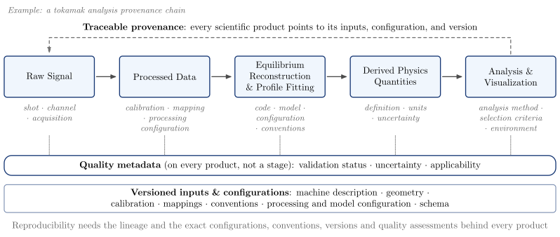
VAFT’s products are designed to be traceable to their inputs, configuration and version. The example below follows one tokamak analysis chain; what is versioned includes the machine description, geometry, calibration, mappings and conventions, the processing and model configuration, and the schema.
| Pipeline | Orchestration | Purpose |
|---|---|---|
automatic_pipeline_1_routine_data_processing |
Snakemake DAG (10 rules) + Makefile |
Per shot: raw DAQ dump → diagnostics/eddy/constraints ODS → EFIT → CHEASE → GPEC suite |
automatic_pipeline_2_corrective_data_update |
Snakemake DAG (8 stages + one replication rule each) | Builds Thomson, CES, core_profiles and the two kinetic EFIT lineages from externally uploaded profile diagnostics |
automatic_pipeline_3_data_summary |
partial Snakefile (2 rules) + manual scripts | Mines the file database into cross-shot .xlsx history sheets and plots |
running_linear_stability |
Snakemake DAG (1 rule, fanned out) | Runs DCON / RDCON / STRIDE per (shot, time, n-mode) on refined equilibria |
All four share one on-disk root, base_dir (/srv/vest.filedb/public in every shipped config), and
pipeline 1 writes under it in one of two layouts selected by the layout: config key.
layout: shot_first (the default) is the legacy server hierarchy, kept so this pipeline stays
directly diffable against the reference output. Its product names are plain .json and stay that
way: the tree is a read-only record of what the legacy pipeline wrote, so it does not follow the
canonical layout’s container (OMAS_PRODUCT_SUFFIX, .json.gz since #813).
{base_dir}/{shot}/
├── diagnostics/          vest_{shot}_daq_raw.json.gz, Thomson *.mat
├── omas/                 {shot}_diagnostics.json, _eddy.json, _constraints.json,
│                         _efit.json, _chease.json
├── efit/                 kfile/ gfile/ afile/ mfile/  + efit_status.txt
├── chease/               refined g-files (flat), work/, plots/{time}.png
├── linear_stability/     {time}/{dcon,rdcon,stride}/nn={n}/
└── logs/
layout: filedb is the canonical grammar (#77), resolved through
vaft.database.filedb.FileDB so no path is reconstructed by hand:
{base_dir}/
├── raw/{shot}/
├── omas/static/{machine_version}/
├── omas/{stage}/{shot}/                          diagnostics, eddy, impa, ...
├── omas/{stage}/{family}/{shot}/                 efit, chease, mhd_linear, gpec_ideal
├── efit/{family}/{shot}/
├── chease/{family}/{shot}/
└── gpec/{family}/{refinement}/{product}/{shot}/n={n}/
with an artifact class (input, output, log, plot, config, work, metadata) as the leaf.
{family} is the reconstruction lineage a product descends from — magnetic, electron or
kinetic; {refinement} is the equilibrium actually handed to the solver (chease, or none); and
{product} is the stability calculation that ran: dcon-peeling, dcon-kink, rdcon, stride or
ideal-gpec. DCON’s two edge treatments are separate products rather than two views of one run,
because a run yields one of them and can never yield both.
To explore what these pipelines actually do – each rule, the files it produces and consumes, the pipeline-1 products pipeline 2 consults, and what each stage publishes to which HSDS source – generated from the Snakefiles themselves, open the pipeline lineage explorer.
Pipeline 1 — routine data processing
Running it
cd workflow/automatic_pipeline_1_routine_data_processing
make run          # snakemake --cores 30 --configfile config.yaml, tee'd into logs/
make clean        # snakemake --delete-all-output
make run hardcodes 30 cores in the Makefile; the cores: key in config.yaml is never read by the
Snakefile. You can equally invoke Snakemake yourself:
snakemake --cores 8 --configfile config.yaml
Two things to know before the first run. make run deletes .snakemake/ when it finishes, so there is no
incremental DAG state between runs — re-execution is decided purely from output-file timestamps. And although
every rule carries a conda: directive, it names a bare environment (vaft) rather than an environment file
and the Makefile does not pass --use-conda; activate the vaft environment yourself.
The DAG
flowchart TD
    A["generate_raw_db_dump<br/>vest_SHOT_daq_raw.json.gz"] --> B["generate_diagnostics_ods<br/>SHOT_diagnostics.json"]
    B --> C["generate_eddy_ods<br/>SHOT_eddy.json"]
    C --> D["generate_constraints_ods<br/>SHOT_constraints.json"]
    B --> D
    D --> E["generate_kfile<br/>efit/kfile/kfiles_generated.txt"]
    E --> F["run_efit_reconstruction<br/>gfiles_generated.txt + efit_status.txt"]
    F --> G["generate_efit_ods<br/>SHOT_efit.json"]
    F --> H["run_chease<br/>refined_gfiles_generated.txt + chease_status.txt"]
    H --> I["generate_chease_ods<br/>SHOT_chease.json"]
    H --> J["run_gpec_suite<br/>gpec_suite_runs.json + gpec_suite_status.txt"]
generate_constraints_ods takes two products, not one. Each stage stores only the IDS it owns,
so the constraint builder reads magnetics, pf_active and tf from the diagnostics product and
pf_passive from the eddy product, unioning them through
vaft.database.composition.compose_stage_products. That composer also refuses a pairing whose time
grids show the two came from different runs — the EFIT constraint builder interpolates each slice
onto pf_passive.time, so a mismatched pairing produces wall currents for the wrong instants
rather than an error.
Stages do not hand individual g-/k-files to each other as Snakemake outputs. Each stage writes a
manifest — a text file with one absolute path per line — and the next stage reads it. run_gpec_suite
instead emits a JSON payload. Alongside each manifest is a one-line status file, e.g.
completed: returncode=0; gfiles=12
skipped: efit.run=false; kfiles=40
partial: refined_gfiles=8; failed=2
| Rule | Script | Key vaft calls |
|---|---|---|
generate_raw_db_dump |
generate_raw_db_dump.py |
vaft.database.init_pool, vaft.database.dump_all_raw_signals_for_shot |
generate_diagnostics_ods |
generate_diagnostics_ods.py |
vaft.machine_mapping.dataset_description, pf_active, spectrometer_uv, barometry, tf, magnetics |
select_impa_shots (checkpoint) |
select_impa_shots.py |
vaft.machine_mapping.impa.impa_expected_fields |
generate_impa_ods |
generate_impa_ods.py |
vaft.omas.vest_upstream.build_impa_ods → vaft.machine_mapping.impa.impa |
generate_eddy_ods |
generate_eddy_ods.py |
vaft.machine_mapping.pf_passive, em_coupling, vaft.omas.process_wrapper.compute_eddy_currents |
generate_constraints_ods |
generate_constraints_ods.py |
vaft.omas.plasma_timing.plasma_timing, vaft.code.efit.correct_flux_loop, vaft.code.efit.generate_constraints_ods |
generate_kfile |
generate_kfile.py |
vaft.code.efit.generate_kfile |
run_efit_reconstruction |
run_efit_reconstruction.py |
vaft.code.efit.run_efit with EFITInputs / EFITConfig |
generate_efit_ods |
generate_efit_ods.py |
vaft.code.efit.collect_efit_outputs |
run_chease |
run_chease_refinement.py |
vaft.code.chease.find_chease_executable, prepare_chease_inputs, run_chease |
generate_chease_ods |
generate_chease_ods.py |
vaft.data.eqdsk.read_geqdsk → .to_omas(ods=ods, time_index=...) |
run_gpec_suite |
run_gpec_suite.py |
vaft.code.gpec.run_gpec_suite_case with GPECCaseInputs / GPECSuiteConfig |
Note the one rule whose name differs from its script: rule run_chease runs run_chease_refinement.py.
generate_impa_ods is the one optional branch. IMPA is an insertable,
campaign-dependent diagnostic, so it is off by default (impa.enable: false),
it is never an input to a baseline stage, and it records a failure in its own
manifest instead of raising one – a broken IMPA branch cannot change the exit
state of a run whose baseline stages succeeded. Its product is published into
the sparse impa HSDS source rather than into main, and a shot missing from
that source means only that no IMPA product was published for it (issue #305).
Analysis that wants the array alongside the baseline composes the two
explicitly with vaft.database.compose(shot).
The library calls, verbatim
Each script is a thin CLI around a handful of vaft calls. These are the load-bearing ones:
from vaft.code.efit import EFITConfig, EFITInputs, run_efit, collect_efit_outputs
from vaft.code.chease import CHEASEConfig, find_chease_executable, prepare_chease_inputs, run_chease
from vaft.code.gpec import GPECCaseInputs, GPECSuiteConfig, run_gpec_suite_case
from vaft.data.eqdsk import read_geqdsk

# EFIT: run, then collect whatever landed in the workdir
result = run_efit(EFITInputs(workdir=workdir, kfiles=kfiles),
                  EFITConfig(executable=exe, workdir=workdir, shot=shot,
                             args=("129",), timeout=3600))
result = collect_efit_outputs(workdir, EFITConfig(workdir=workdir, shot=shot))

# CHEASE: resolve the binary ($CHEASEHOME/bin/chease, then $CHEASE,
# then $CHEASE_EXEC_DIR -- there is no $PATH fallback), prepare, run
# GEQDSK in, GEQDSK out: the adapter selects CHEASE's NIDEAL itself (#516)
config = CHEASEConfig(executable=exe, timeout=600, target_psin=0.993, nw=513)
result = run_chease(prepare_chease_inputs(gfile, config), config)

# GPEC suite: one case per refined g-file
result = run_gpec_suite_case(
    GPECCaseInputs(shot=shot, time_ms=time_label, geqdsk=gfile, workdir=workdir),
    GPECSuiteConfig(gpec_home=gpec_home, modules=("dcon", "rdcon", "stride", "gpec"),
                    modes=(1, 2), psilow=0.01, psihigh=0.994, timeout=1200.0))

# CHEASE ODS: accumulate refined g-files as time slices
ods = read_geqdsk(gfile).to_omas(ods=ods, time_index=time_index)
GPECSuiteConfig.gpec_home defaults to None, in which case the installation root is read from the
$GPECHOME environment variable.
The diagnostics stage forces the machine-mapping layer offline by setting VAFT_RAW_SAMPLE_PATH and
VAFT_RAW_OFFLINE_ONLY=1 before it maps anything, so the whole pipeline can be replayed from an archived raw
dump with no SQL server in reach. Magnetics processing parameters travel as a
vaft.process.magnetics.VestMagneticsProcessingConfig, built from the vest.magnetics.processing block of
config.yaml and passed to vaft.machine_mapping.magnetics(..., processing_config=...). See
Signal processing and EM modeling for what those knobs mean.
Configuration
config.yaml is organised by stage: raw (mode: sql | archive), diagnostics (tstart, tend, dt,
run), vest.magnetics.processing, wall.reference_ods, eddy.filament (r, z, fraction, dt_sub),
constraints, efit, chease and gpec. Three points repeatedly bite newcomers:
- The shipped
config.yamlis a template, not a working config.efit.executable,efit.table_dir,chease.executable,gpec.home,wall.reference_odsandraw.archive_templateall point into one developer’s home directory, whilebase_dirpoints at the Linux data server. Repoint them before running. - Dead keys.
cores,raw.offline_onlyandgpec.coil.sourceappear inconfig.yamlbut are never read by theSnakefile. - Channel selection is a decision the constraint stage consumes, not one it makes (issue #296).
vaft.validation.efit_channels.decide_efit_channelsreads the validity the diagnostics stage projected and emits a per-channel, per-slice decision — usable, suspect, rejected, missing or recovered — thatgenerate_constraints_odsonly translates into weights. There is no manual channel list any more (issue #295 retiredconstraints.broken; its evidence is inworkflow/efit_channel_selection/README.md), so a channel is a constraint unless the assessment says otherwise.constraints.detect_broken: truenow means require that assessment: a product without projected validity is refused and must be re-run through the diagnostics stage (withfalseevery channel is usable by default). No detector runs in this stage.gaussian_fit_optionselects the compatibility recovery backend (1refits rejected probes from their family’s Gaussian profile,2every probe); a recovered value never re-enables a channel the quality layer rejected. The decisions are recorded in the product underequilibrium.code.parameters.channel_decisions. efit.presetselects a named EFIT configuration fromvaft.code.efit.PRESETS: empty is the library default (statistical_891, since 2026-10-01) androutinethe legacy one. The k-file stage always writesefit_preset.jsonbeside its manifest and the EFIT product carries that record undercode.parameters(efit_collection.efit_preset); pipeline 2’skinetic.efit_presetbuilds the kinetic lineages’ base magnetic k-file the same way. Aroutinerun writes the same product paths as a default one, so give it its ownbase_dir. What each preset sets is tabulated under Named configurations.
Each constraint is the box average of the diagnostic samples inside [t_i − w, t_i + w] — every
sample once, equal weights, no interpolation grid of its own (issue #433) — with w =
constraints.average_window (0.5 ms by default). The window and the reconstruction cadence tstep are
two separate controls; qualifying them together is issue #468.
Constraint time selection is worth spelling out, because timeset: auto is the default and it is not
obvious. The script takes the shared plasma-analysis range — diagnostics_time_policies.windows.plasma_analysis
in vest.yaml, 0.28–0.36 s — and intersects it with the plasma window vaft.omas.plasma_timing detects on
the product: the slow H-alpha line found by label, else the validated fast line, else the plasma-current
principal pulse (see Plasma timing policy).
When no source shows a plasma the whole range is used and the run is flagged analysis_range_fallback,
with the reason, in the stage log and in equilibrium.ids_properties.comment, which always names the
window and its source. Start and end are clamped to tstart/tend when given and snapped to the tstep
grid, and the end instant is included. With timeset: manual you get exactly np.arange(tstart, tend, tstep)
and both bounds become mandatory.
Failure semantics — a green run does not mean everything ran
The runners deliberately disagree about what counts as failure, so always read the *_status.txt files
rather than the exit code:
run_efit_reconstructionandgenerate_efit_odsexit 0 even when EFIT is absent or produced nothing. A minimal stub ODS is written instead, carryingequilibrium.ids_properties.comment = "EFIT output unavailable: ...". Check that comment to detect a stub.- EFIT failure is detected by string-sniffing stdout and stderr for
Invalid line in namelist,Fortran runtime errorandError termination— EFIT is known to exit 0 on namelist errors, so the return code alone is not trustworthy. run_chease_refinementexits 1 if CHEASE ran but refined zero g-files (though 0 if it was skipped outright), andrun_gpec_suiteexits 1 if any case failed.
run_chease_refinement.py also writes chease/chease_runs.json and the per-time comparison plots in
chease/plots/, neither of which is declared as a Snakemake output — snakemake --delete-all-output will
leave them behind.
Pipeline 2 — corrective data update
This pipeline builds the products that depend on data uploaded after a shot was processed: Thomson
scattering, charge exchange (CES), the core_profiles mapped from them, and the two kinetic EFIT lineages.
It is a Snakemake stage-product DAG, like pipeline 1. The composition stage then adds the assumed impurity
composition, the diluted ion density and Z_eff(rho) to the measured profiles.
cd workflow/automatic_pipeline_2_corrective_data_update
snakemake --snakefile Snakefile --configfile config.yaml --cores 8
config.yaml ships with base_dir: /srv/vest.filedb, shots: [48226] and layout: filedb. Only the
canonical filedb layout is accepted; these stages have no shot-first equivalent. external.data_root is
where the hand-uploaded .mat files are searched for, external.ces_options picks the ion layout (ces for
CES_{shot}.mat, ids for IDS_{shot}.mat), and kinetic.* selects the pressure-point encoding, the EFIT
executable and the named EFIT preset used for the base magnetic k-file.
Stages
| Stage | Builder (vaft.omas.vest_upstream) |
Needs | Replicated IDS and source |
|---|---|---|---|
thomson |
build_thomson_ods |
an uploaded Thomson file | thomson_scattering → main |
ces |
build_ces_ods |
an uploaded CES file | charge_exchange → main |
core_profiles |
build_core_profiles_ods |
thomson (+ ces), pipeline 1’s EFIT |
core_profiles → main |
composition |
build_composition_ods |
core_profiles, pipeline 1’s EFIT and diagnostics |
core_profiles → main, after the stage above |
ti_inferred (opt-in) |
build_ti_inferred_ods |
composition, pipeline 1’s magnetic EFIT |
core_profiles → main, after composition |
resistive_zeff (opt-in) |
build_resistive_zeff_ods |
ti_inferred, pipeline 1’s magnetic EFIT |
core_profiles → main, after ti_inferred |
electron_efit |
build_kinetic_efit_ods |
composition (else core_profiles) without ion data |
equilibrium → electron-efit |
kinetic_efit |
build_kinetic_efit_ods |
composition (else core_profiles) with ion data |
equilibrium → kinetic-efit |
Pipeline 1’s EFIT and constraints products are passed to these rules as params, not input: a shot that
pipeline 1 never reconstructed is then recorded as unavailable instead of making Snakemake raise. Which of
the two kinetic lineages runs for a shot is decided by whether a core_profiles slice carries a measured ion
temperature (read from its fit record; the assumed T_i = T_e of composition and an inferred T_i do not
count), not by configuration. The destinations come from STAGE_REPLICATION in
vaft/database/sources.py; the two kinetic lineages go to their own sources because they share the
equilibrium IDS with the baseline EFIT.
The composition overlay
composition takes the measured core_profiles product and adds, per slice, the C/O composition of
machine_mapping/vest.yaml’s impurity_model (equal carbon and oxygen elemental densities, n_e dV-mean
Z_eff = 2): ion[] with charge states, the diluted main ion and zeff. Everything it writes is an assumption
(origin=assumed|derived in the *_fit.parameters record, with target_zeff=), and a zeff labelled measured is
never overwritten. Each composed slice also records the equilibrium it was matched to
(equilibrium_lineage=magnetics; equilibrium_occurrence=0; equilibrium_time_s=...) in its electron temperature
fit record and, when it has an ion temperature, in that record.
ionization(composition.ionization, defaulttransient) needs the plasma age,t - onset, with the onset fromplasma_timingon pipeline 1’s diagnostics product. A slice with no positive age is skipped and named in the manifest rather than silently computed ascoronal, which overstates the charge on VEST’s short discharges.- ADF11 atomic data come from OPEN-ADAS and are fetched on first use. A server without network needs the cache
warmed and
composition.adf11_cache_dirpointing at it. - Pressure counts the diluted ions. The composed slice’s
pressure_thermalis recomputed with the species kinetic closure (infer_kinetic_closure), so it no longer counts one ion per electron: a measuredT_igiveselectrons.pressure,pressure_ion_totalandpressure_thermal; a slice with noT_igets the electron pressure only; aT_ithe product assumed keeps the pressure it was written with. The closure is named inion.0.density_fit.parameters(pressure_closure=infer_kinetic_closure; dilution=species). - Replication is an overlay.
core_profilesandcompositionboth own thecore_profilesIDS inmain, which the registry otherwise avoids. Thecompositionreplication waits for thecore_profilesrecord, somainholds the composed product when the stage succeeded and the measured one when it was skipped.
The inferred ion temperature
The default scope does not build ti_inferred or resistive_zeff: main gets ⟨Z_eff⟩ = 2 and, on slices with no measured T_i, the stated assumption T_i = T_e from composition (#1842; on the Tier A shots the pressure partition returned T_i/T_e ≈ 2 and the resistive Z_eff was identifiable on few shots). Name the stages in stages to build them; ti_inferred replaces an assumed T_i, never a measured one.
ti_inferred gives the slices that have no measured T_i an ion temperature from the pressure partition of
pipeline 1’s magnetic EFIT: T_i = p_eq / (e f n_e) - T_e / f, with p_eq sampled on the slice’s own flux surfaces
and f = n_i,tot / n_e the composed product’s diluted ion density
(vaft.process.kinetic_closure.infer_ti_pressure_partition, which moved there from
vaft.validation.kinetic_state and keeps a warning alias in the old place).
- Inferred, never measured. The ion records say
origin=inferred; method=equilibrium_pressure_partitiontogether withequilibrium_lineage,equilibrium_occurrence,equilibrium_time_s,sigma_p_eq_basisandvalid_points;classify_ti_recordreads them back asinferred. Points wherep_iis not positive and significant stay NaN (flagged, never filled), andt_i_average,pressure_ion_totalandpressure_thermalfollow:p_thermalequals the equilibrium pressure there by construction, a closure identity and not an agreement test. - Only the magnetic lineage. The lineage is read from where the EFIT product lives (
omas/efit/magnetic), never asserted; a pressure from elsewhere is refused. The electron-kinetic EFIT was fitted with an assumedT_i/T_eand would return that assumption. For the same reasonti_inferredis a leaf: the kinetic EFIT stages readcomposition, never this product. sigma(p_EFIT)is the spread over the usable neighbouring slices withinti_inference.window_s, floored atti_inference.floor(0.17, #874) of the pressure;n_eandT_etake the Thomson channels’ median relative error.- Skipped, and named, rather than guessed: a slice with a measured
T_i, with no composition (the ion density is half the formula), with no equilibrium within the tolerance, or with no significant point. - On the archived 40326 / 322 ms case the stage reproduces the notebook’s
T_ito 1e-14 wherever both are valid, and voids 8 more edge points (rho_tor_norm > 0.86) because it carries a differentsigma(p_EFIT).
The resistive Z_eff
resistive_zeff stores Lane Z’s Romero estimate (issue #1214) in
core_profiles.global_quantities.z_eff_resistive, beside the composition Z_eff (profiles_1d.zeff) and never over it.
Romero’s transformer balance over the current-carrying window of the magnetic EFIT (boundary flux, I_p, l_i) gives the
observed plasma resistance; the one Z_eff that makes the conductivity model, run on each kinetic slice’s T_e, n_e
and Grad-Shafranov geometry, match it is the estimate. The physics is Lane Z’s (vaft.omas.resistive_zeff,
vaft.process.resistive_zeff); this stage orchestrates it.
- A window scalar, not a per-slice value. One slice carries the full noise of a differentiated
V_R, so the estimate is a single number for the window (#1214 Sec. 9): it is written at every usable kinetic slice and is NaN elsewhere. The per-slice solutions are in the manifest as a labelled diagnostic and are not stored in the IDS. An estimate that sits on a bound (bound_hit), or is not identifiable, is recorded and not stored. - Stated settings. The estimator has no defaults:
resistive_zeff.model(redl),ln_lambda(sauter),bounds(1-8),i_ni_a(0, a purely Ohmic window),smoothing(none) and the two state filters (a state with more than 5 % ofj_toroutside its profiles, or|V_I|/|V_B| >= 1, is dropped) are config and are recorded in the product. - Provenance is
resistive_*fields in the slice’szeff_fit.parameters(resistive_origin=inferred,resistive_model=romero_transformer,resistive_conductivity,resistive_window,resistive_status,resistive_sigma,resistive_equilibrium_lineage,resistive_equilibrium_occurrence,resistive_i_ni_a,resistive_smoothing): prefixed so they cannot be read as the composition record’sorigin/method. - Cross-check. The manifest turns the stored composition
Z_eff(rho)into the scalar the same estimator would report were it the truth (vaft.process.zeff_projection) and compares it with the estimate (crosscheck: the equivalent, the difference and the relative difference). It needs a real toroidal-flux coordinate: with thesqrt(psi_N)proxy inrho_tor_normit is withheld and says why, and the estimate still stands. - Only the
efit/magneticlineage is accepted (read from where the product lives), as forti_inferred. It is a leaf.
Dilution in the kinetic EFIT
Both kinetic lineages read the composition product (the measured one itself when composition was skipped, so they
never depend on its outcome). With kinetic.dilution: species (the default) the raw pressure points are
p = e n_e (T_e + f T_i) with f = n_i,tot / n_e at each Thomson radius, from the stored ions; the spline encoding
gets the same through pressure_thermal. f is an assumed composition and is not added to SIGPRE. The effect is
f - 1 times the ion term: about 2-3 % of the pressure where T_i/T_e ~ 0.15 (48224), and up to ~8 % for the assumed
T_i = T_e of electron_efit. A slice with no composition falls back to n_i = n_e; the manifest dilution block
and equilibrium.code.parameters (kinetic_efit.dilution) say which was used and why. kinetic.dilution: none restores
the legacy pressure.
Reading the result
Every stage always writes a product and a manifest and exits 0; read the manifest status, not the exit code.
| Manifest status | Meaning | Replicated? |
|---|---|---|
success (also partial, completed) |
the stage produced its product | yes |
unavailable |
the upstream data does not exist for this shot (the normal case for most shots) | no — recorded as skipped |
no_output |
the stage ran and had nothing to write | no — recorded as skipped |
failed |
the builder raised; the product is an empty ODS | no — recorded as skipped |
All five stages are optional, so a skipped replication does not change the pipeline’s exit state.
hsds.replicate: true adds one replicate_<stage>_to_hsds rule per stage; each stage owns only its own IDS,
and readers union the stages explicitly with vaft.database.composition.compose_stage_products.
The legacy daemons and the registry
The pre-Snakemake implementation — three polling scripts that wrote the shot-first public/ tree and the
HSDS registry processed_shots.h5 — is quarantined under workflow/automatic_pipeline_2_corrective_data_update/legacy/
with its own README. It is not part of the supported pipeline and must not be run against main.
The registry is therefore no longer maintained. vaft.database.exist_shot(data_filter='ts'|'cx'|'cp') still
reads whatever the old daemons left in it, and returns None for a source that never had one; treat it as a
historical record. Pipeline 3 does not use it: its generators list shots with
vaft.database.exist_shot(source=..., strict=True) (no filter) inside vaft.database.summary, i.e. the shots
present in the named HSDS source.
Running it unattended
vaft corrective-worker watches the upload directory (external.data_root) and runs this pipeline for a shot when
an upload for it appears or changes and has been quiet for quiet_seconds. It is independent of
vaft pipeline-worker (its own state file, lock and run directories), judges each shot by the stage manifests of the
stages in scope (stages; unavailable and no_output are results, failed is retried), forces the rerun of a
changed or failed shot (the root rules have no input files, so Snakemake would otherwise call it up to date), and stops
starting runs while its hold_file exists, which is how it stays off shots a regeneration owns. It does not notice a
change in pipeline 1’s products. Each stage also has an optional validation figure set (plots.enabled) that the worker
does not judge. See workflow/automatic_pipeline_2_corrective_data_update/DEPLOYMENT.md.
There is no era table or static product for this pipeline: the machine era enters through vest.yaml (the impurity
model and the Thomson/CES mappers), not through a per-era product.
Pipeline 3 — data summary
Cross-shot mining. The Snakefile here wires up only two of the ten-odd scripts (with BASE_PATH hardcoded,
not read from a config — config.yaml and README.md are both empty files); everything else is run by hand.
cd workflow/automatic_pipeline_3_data_summary
snakemake --cores 8                                   # chease_history.xlsx + efit_history.xlsx
python gen_omas_history.py     --base-path /srv/vest.filedb/public
python gen_stability_history.py --base_path /srv/vest.filedb/public   # underscore!
python gen_core_profiles_history.py --directory public --Z-eff 2.0 --save-every 10
python gen_equilibrium_global_history.py --directory public --rebuild
python gen_volume_averaged_parameter_sheet.py --max-shots 50 --directory public
| Script | Sheet | Contents |
|---|---|---|
gen_chease_history.py |
chease_history.xlsx |
Global quantities per (shot, time) from refined g-files |
gen_efit_history.py |
efit_history.xlsx |
Same columns from EFIT g-files (key column is shot_number, not shot) |
gen_omas_history.py |
omas_history_new.xlsx |
One row per shot: onset, pulse duration, peak $I_p$, $B_t$, file-existence flags |
gen_stability_history.py |
stability_history.xlsx |
Ideal/resistive/ballooning classification per (shot, time) |
gen_core_profiles_history.py |
core_profiles_history.xlsx |
$\tau_E$ and confinement scalings per time slice: the legacy modelled p_loss_MW/tau_e_s and the measured-loop Ohmic v_res_V, p_ohm_MW, p_net_MW, w_mhd_kJ, tau_e_net_s side by side (CORE_PROFILES_DEFINITIONS, #1905) |
gen_equilibrium_global_history.py |
equilibrium_global_history.xlsx |
50+ columns: globals, geometry, diamagnetic flux, virial/Shafranov block |
gen_volume_averaged_parameter_sheet.py |
volume_averaged_parameters.xlsx |
$\langle n_e \rangle$, $\langle T_e \rangle$, $\langle P_e \rangle$ vs. $\langle P_{eq} \rangle$ |
join_chease_stability_history.py |
chease_stability_history.xlsx |
Inner-join of the CHEASE and stability sheets on ['shot', 'time [ms]'] |
plot_stability_limit.py |
stability_limit.png, histograms.png, corr/*.png |
Stability-limit scatter, histograms, pairwise correlations |
The equilibrium and profile generators lean on the ODS-aware layer described in
Data structures, calling vaft.omas.update_equilibrium_boundary,
update_equilibrium_global_quantities_q_min, update_equilibrium_global_quantities_volume,
update_equilibrium_stored_energy and update_equilibrium_constraints_diamagnetic_flux to fill any gaps,
then vaft.omas.compute_virial_equilibrium_quantities_ods and
vaft.omas.compute_diamagnetic_flux_measured_vs_computed for the derived blocks. Confinement times come from
vaft.omas.formula_wrapper.compute_tau_E_engineering_parameters together with
vaft.omas.general.find_matching_time_indices, which pairs a core_profiles slice with the nearest
equilibrium slice. Volume averages use vaft.omas.update_core_profiles_global_quantities_volume_average and
vaft.omas.compute_volume_averaged_pressure(ods, time_slice=None, option="equilibrium").
gen_core_profiles_history.py, gen_equilibrium_global_history.py and
gen_volume_averaged_parameter_sheet.py share an incremental-upsert engine: they reload the existing sheet,
reprocess any shot that is missing or defective (any required column NaN or non-finite), upsert on the key
columns, and checkpoint every --save-every shots. --rebuild ignores the existing sheet entirely. The other
generators rebuild from scratch and overwrite.
Reading these sheets correctly
- The stability classifications are heuristics with magic thresholds.
ideal_stabilityis"Error"if any $|\delta W| \ge 100$, else"Stable"only if every $\delta W > 0$ (scanned over $n = 1 \ldots 6$).resistive_stabilityis"Error"if any $|\Delta’| \ge 1000$, else"Stable"if no $\Delta’ > 0$ ($n = 1, 2$).ballooning_stabilityis"Unstable"if $c_{a1} < 0$ anywhere with $\psi_N > 0.5$. Thesas_flagvalues are parsed from the code input files but dropped from the final sheet. chease_history.xlsxis indexed by PNG files, not g-files. Discovery enumerateschease/plots/*.pngand derives the time from the stem. Setchease.create_plot: falsein pipeline 1 and this sheet comes out empty even with hundreds of valid refined g-files present.- There is no canonical schema across sheets. The key column is variously
shot,shot_numberorshotnumber, and the time columntime [ms],time,time_sortime_ms. That is whyjoin_chease_stability_history.pycan join the CHEASE sheet but not the EFIT one. gen_chease_history.pyappliesabs()to $I_p$;gen_efit_history.pydoes not, so EFIT currents can come out negative.- The filename chains do not compose.
gen_omas_history.pywritesomas_history_new.xlsxbutplot_omas_history.pyreadsomas_history.xlsx;join_chease_stability_history.pywriteschease_stability_history.xlsxbutplot_stability_limit.pyreadschease_dcon_history.xlsx. Rename or copy by hand between steps. - Despite their names,
plot_chease_history.pyandplot_efit_history.pydo not plot. Both are older generators;plot_chease_history.pyin particular overwriteschease_history.xlsxwith an incompatible schema that can no longer be joined. Do not run it.plot_stability_history.pyis an empty file. gen_efit_reliability.pycurrently emits only diamagnetic-flux rows — the append calls in its magnetic-probe and flux-loop branches are unreachable — so do not read its output as per-probe reliability data.
running_linear_stability
Pipeline 1’s run_gpec_suite rule runs the GPEC suite through the vaft.code.gpec API. This separate
pipeline is the older, coarser alternative: a fan-out that launches DCON, RDCON and STRIDE directly, one
Snakemake job per (shot, time, code, n-mode). For what these codes compute and how to read their output, see
Stability.
cd workflow/running_linear_stability
./snakemake_worker.sh          # snakemake --cores 28
Targets are discovered by find_plotted_gfiles.py, which the Snakefile shells out to at parse time. It
walks {BASE_DIR}/{5-digit shot}/chease/plots/*.png, takes each PNG stem as a 5-digit time, and emits the
matching chease/g{shot:06d}.{time} — the same PNG-as-index coupling as gen_chease_history.py, so
CHEASE comparison plots must exist or this pipeline finds nothing to do. You can run the discovery step alone:
python find_plotted_gfiles.py --base-path /srv/vest.filedb/public
The single rule run_stability_code_for_mode fans out over $n = 1 \ldots 6$ for DCON and $n = 1, 2$ for RDCON
and STRIDE, writing a completed.txt marker to
{BASE_DIR}/{shot}/linear_stability/{time}/{code}/nn={n}/ and a log to
{BASE_DIR}/{shot}/logs/linear_stability/{time}/{code}_nn{n}.log. That directory layout is exactly what
gen_stability_history.py in pipeline 3 later reads.
Two caveats. The rule loads GPEC through environment modules (module use /home/user1/GPEC/module; module load
GPEC-dev), and the runner it invokes is an absolute path to a script outside this repository
(RUN_PARALLEL_DCON_SCRIPT at the top of the Snakefile). Both must be repointed for the pipeline to run
anywhere else. config.yaml holds a single key, BASE_DIR.
To wipe stability outputs and start over — inspect first, it is a recursive delete:
python cleanup_stability_outputs.py --base-path /srv/vest.filedb/public --dry-run
python cleanup_stability_outputs.py --base-path /srv/vest.filedb/public
It removes {shot}/linear_stability/ and {shot}/logs/linear_stability/ for every shot under the base
path.
Related
Each pipeline stage has an interactive notebook counterpart — read those first if you want to understand what a stage does before running it at scale:
magnetic_diagnostics_processing.ipynbandeddy_current_calculation_and_startup_analysis.ipynb— pipeline 1, diagnostics and eddy stagesmagnetic_equilibrium_reconstruction_with_efit.ipynbandequilibrium_refinement_using_chease.ipynb— the EFIT and CHEASE stageslinear_ideal_stability_analysis_with_dcon.ipynb,linear_resistive_stability_analysis_with_rdcon.ipynbandperturbed_equilibrium_and_3d_response_with_gpec.ipynb— the stability codesprofile_fitting_using_equilibrium_and_kinetic_diagnostics.ipynbandconfinement_time_scaling.ipynb— pipelines 2 and 3
Guide pages: Installation · Database · Data structures · Machine mapping · Signal processing and EM modeling · Equilibrium · Stability · Physics formulas · Examples
Pipeline sources:
workflow/ ·
vaft/code/efit.py ·
vaft/code/chease.py ·
vaft/code/gpec.py