Scientific diagrams
vaft.diagram draws concepts: topology, coordinate systems, workflows. It does not draw data. The
three layers split the work:
| Layer | Owns | Example |
|---|---|---|
vaft.formula |
the physics: every equation a diagram depends on | helical_phase, island_pendulum_hamiltonian |
vaft.diagram |
explanatory geometry: sampling, projection, camera, labels | magnetic_island(projection="3d") |
vaft.plot |
data and numerical results from an ODS | equilibrium_2d_profiles |
A diagram never restates an equation. It calls the formula function, so the picture and the formula reference cannot drift apart.
This page explains the diagrams family by family. The complete list – every builder, every committed SVG and the exact call that draws it – is the generated diagram gallery.
Magnetic island
import vaft

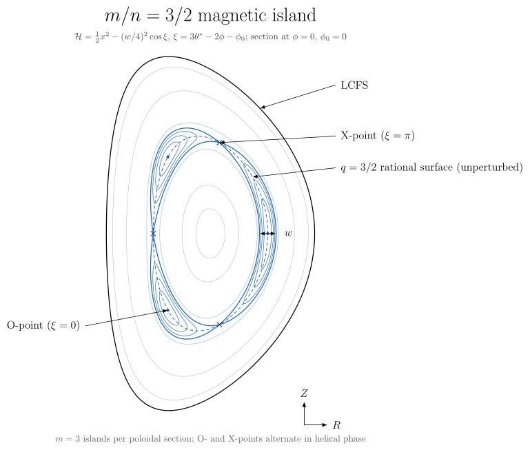
d = vaft.diagram.magnetic_island(
    m=3, n=2, width=0.16, phase=0.0, projection="poloidal",
    r_s=0.55, elongation=1.7, triangularity=0.4,   # D-shaped plasma; defaults give a circle
)
d.tikz       # the LaTeX/TikZ source; needs no TeX installation
# With latex and dvisvgm installed:
# d            -> displays inline in Jupyter (SVG)
# d.save("island.svg")
| Projection | Poloidal section at $\phi=0$ | Top view $(R,\phi)$ | 3-D view of the O and X helices |
|---|---|---|---|
 |
 |
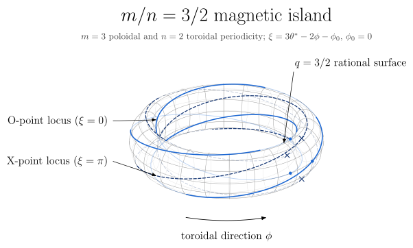 |
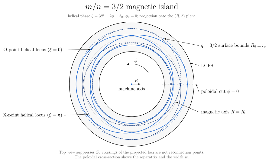
All three views are drawn from one model, and the convention is the same in each:
| Quantity | Definition |
|---|---|
| helical phase | $\xi = m\theta^* - n\phi - \phi_0$, where $\theta^*$ is the straight-field-line (PEST) angle of each surface, running from the outboard midplane towards the top, and $\phi$ runs counter-clockwise seen from above |
| straight-field-line angle | $\theta^* = 2\pi\int \mathcal{J}/R^2\,d\theta / \oint \mathcal{J}/R^2\,d\theta$ (vaft.formula.straight_field_line_angle), taken from the surface geometry alone. O- and X-points are evenly spaced in $\theta^*$, so they spread out on the low-field side even on circular surfaces |
| flux function | $\mathcal{H}(x,\xi) = \tfrac12 x^2 - (w/4)^2\cos\xi$, with $x = r - r_s$ |
| O-points / X-points | $\xi = 0$ (minimum of $\mathcal{H}$) / $\xi = \pi$ (saddle): $m$ of each per poloidal section, alternating |
| separatrix | $\mathcal{H} = (w/4)^2$, so $x_\mathrm{sep} = \tfrac{w}{2}\lvert\cos(\xi/2)\rvert$ |
width |
the full radial width at the O-point, in units of the minor radius |
| geometry | Miller shaping from vaft.formula.miller_surface: $R = R_0 + r\cos(\theta + \arcsin\delta(r)\,\sin\theta)$ and $Z = \kappa r\sin\theta$, with $\delta(r) = \delta\,r$ so the surfaces stay nested and become circular towards the axis. Lengths are in units of the minor radius $a$ |
| caveats | The surfaces are prescribed, with no Shafranov shift, so $\theta^*$ is exact for these surfaces rather than for a Grad-Shafranov equilibrium. width is a width in the flux label $r$ and is a physical distance only on the outboard midplane |
The top view suppresses $Z$, so crossings of the projected O and X loci there are not reconnection points. The separatrix and $w$ are only visible in the poloidal section.
Animating the island: a phase scan or a rigid rotation
The same call draws the island over a trajectory of its phase when it is asked to with
animation=True (issues #1049, #1053). It returns the animation result that
plot_*(..., animation=True) returns. An array argument never animates by itself.
import numpy as np
import vaft

# A helical-phase scan: one frame per phi_0, the same model as the static call.
scan = vaft.diagram.magnetic_island(m=2, n=1, phase=np.linspace(0, 2 * np.pi, 120), animation=True, fps=30)
scan.save("island.mp4")          # or .webm (both need vaft[video]) or .gif (needs nothing)

# A rigid rotation at f = 5 kHz: phi_0(t) = phi_0 + 2*pi*f*(t - t_0), from phase= at the first time.
rotation = vaft.diagram.magnetic_island(
    m=2, n=1, time=np.linspace(0, 2e-3, 120), rotation_frequency=5e3, animation=True,
)
rotation.metadata["driver"]      # name "time", unit "s", and every frame's time
- Exactly one trajectory. A trajectory is either
phaseas an array (driverphase[rad]) ortimewithrotation_frequency(drivertime[s]).- A phase array combined with
timeis refused, because it is ambiguous. - So is a single phase with
animation=True, which is a static diagram.
- A phase array combined with
- Units and direction.
rotation_frequencyis a frequency $f$ in Hz. The synthetic island of #886 (vaft.process.magnetic_island.MagneticIslandSpec) takes the angular frequency $\omega = 2\pi f$ in rad/s. A positive $f$ moves the O-points towards $+\theta^$ on a section. At fixed $\theta^$, it moves them towards $-\phi$, which is clockwise seen from above. - Physics, not pictures. Every state is the static diagram at that phase, with the same O/X topology, width and shaping. The rotation is the phase relation evaluated at each time; the drawing is never rotated as an image.
- Presentation only.
fpsordurationset only how fast the frames are shown, never the rotation rate. Each frame’s phase or time is kept inmetadataand in the.jsonsidecar ofsave(). - A preview of the canonical figure. The frames are a Matplotlib drawing of each state’s scene (the template’s colours and line styles, with labels through mathtext). The canonical static figure remains the SVG above.
Stability and operational-space diagrams
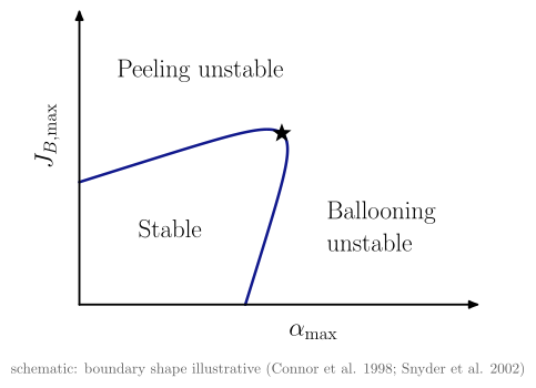
Textbook 2-D charts: two axes, the boundaries that divide the plane, and one label per region. A
boundary that physics defines is computed by vaft.formula. Only the peeling–ballooning boundary,
which has no closed form, is a schematic, and the figure says so.
vaft.diagram.peeling_ballooning()
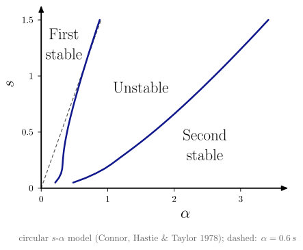
vaft.diagram.s_alpha_ballooning(s_max=1.5, alpha_max=3.5)
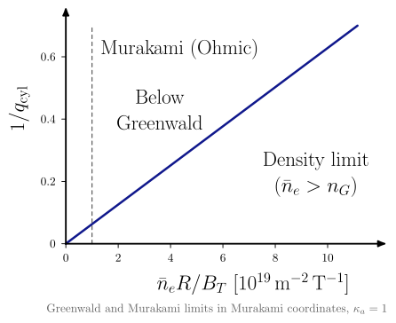
vaft.diagram.hugill(elongation=1.0)                       # no size parameter: R, a, B cancel
vaft.diagram.hugill_st(elongation=1.8)                   # spherical-tokamak q_cyl (Sykes et al. 2000, MAST)
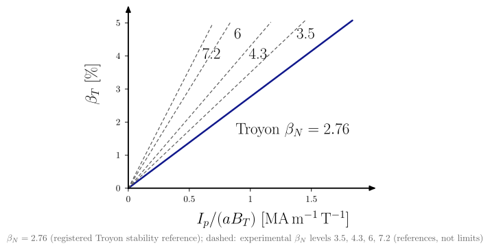
vaft.diagram.troyon(aspect_ratio=3.0, elongation=1.7)      # Troyon stability reference ~2.76, experimental levels dashed
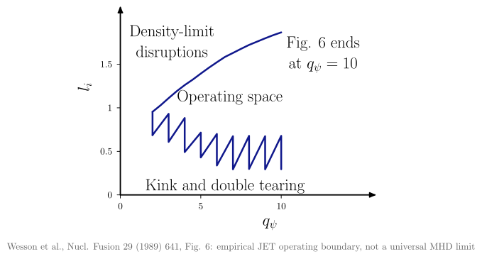
vaft.diagram.li_qa(reference="wesson_1989")                # JET empirical l_i-q_psi space
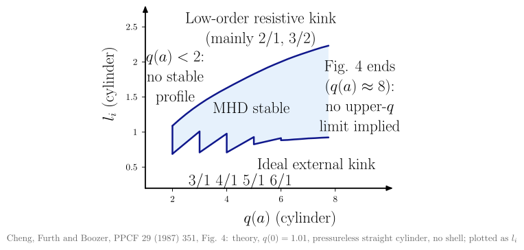
vaft.diagram.li_qa(reference="cheng_1987")                 # theoretical MHD-stable l_i-q(a) domain
 |
 |
 |
 |
 |
 |
| Diagram | Question it answers | Axes | Boundaries |
|---|---|---|---|
| Peeling–ballooning | Which edge instability limits the pedestal? | $\alpha_\mathrm{max}$, $J_{B,\mathrm{max}}$ (arbitrary units) | Schematic. Two linear margins joined by a smooth maximum. The ★, where the peeling and ballooning limits meet (typical ELM onset), is computed where the two margins are equal |
| $s$–$\alpha$ | How does shear set the ballooning limit, and where is second stability? | $\alpha$, $s$ | The first and second stability boundaries come from s_alpha_marginal_alpha, which applies Newcomb’s criterion to the Connor–Hastie–Taylor equation. The dashed line is the $0.6\,s$ approximation of ballooning_stability_criterion. Not resolved below $s \approx 0.05$ |
| Hugill | Where is the density limit? | $\bar n_e R/B_T$, $1/q_\mathrm{cyl}$ | The registered greenwald_hugill line (slope $\pi/50\kappa_a$ in $1/q_\mathrm{cyl}$ against $\bar n_e R/B_T$) and murakami_hugill ($\bar n_e R/B_T = 1$). The registered low_q is on the equilibrium $q_\psi$, not $q_\mathrm{cyl}$, so it is not drawn; q_limit= adds a dashed reference $q_\mathrm{cyl}$ line |
| Hugill (ST) | Where is the density limit in a spherical tokamak? | $\bar n_e R/B_T$, $1/q^{ST}\mathrm{cyl}$ with $q^{ST}\mathrm{cyl} = 2.5a^2(1+\kappa^2)B_T/(RI_p)$ | vaft.diagram.hugill_st(elongation=1.8): the Hugill limit as Sykes et al. (2000, MAST) define it (sykes_2000_st_hugill) and the Greenwald limit on these axes (greenwald_hugill_st, derived); Murakami dashed as a historical conventional-tokamak reference. Not substitutable with the conventional hugill axes (#1602) |
| $l_i$–$q$ | Where do current-profile peaking and edge q allow stable operation? | Wesson: $q_\psi$, $l_i(3)$. Cheng: cylinder $q(a)$, $l_i$ | Two separate references, never mixed. Wesson 1989 Fig. 6: the JET empirical boundaries (kink and double tearing below, density-limit disruptions above), with the registered low_q closing $q_\psi = 2$. Cheng 1987 Fig. 4: the theoretical MHD-stable domain of a cylinder with $q(0) = 1.01$ (ideal kink below, resistive kinks above), plotted as $l_i$ rather than $l_i/2$ |
| Troyon | How much pressure has the current held, against which references? | $I_p/(aB_T)$, $\beta_T$ | The registered troyon stability reference, $\beta_N = 2.2\,\mu_0 10^6 \approx 2.76$, through $\beta_T = \beta_N I_p/(aB_T)$, with the experimental $\beta_N$ levels of the troyon projection dashed (DIII-D envelope and record, ST reference, NSTX record; #1691). None is a limit, so no side is shaded or called stable. beta_N_max= draws a what-if value and the note says so; q_limit= adds a dashed reference $q_\mathrm{cyl}$ cutoff |
These charts show the boundaries of an operating space. Each one reads its lines from
vaft.formula.boundaries through a canonical projection (#1425), and a population of measured or
modelled states goes on the same projection with
vaft.plot.operational_space.operational_space_population(table, "hugill"). Table columns are named
by quantity identity (murakami_parameter, inverse_cylindrical_q, normalized_beta, …) with
units in table.attrs["units"]. A boundary is drawn only when both plotted columns are exactly the
projection’s quantities in its units: a q95 column never carries a $q_\psi$ or $q_\mathrm{cyl}$
boundary. Projections: hugill, troyon, beta_n_li, q95_li, greenwald_fraction_power,
li_qa_wesson, li_qa_cheng, beta_n_li1 (Strait’s $\beta_N = 4\,l_i(1)$ envelope), and the #1691 beta-normalisation views volume_beta_in,
beta_n_normalizations (with a $y = x$ guide), aspect_ratio_beta_n, aspect_ratio_volume_beta_n;
list_projections() gives the full set. See
#944 and #636.
Dimensionless similarity spaces
The limit diagrams above ask whether a state crosses a boundary. A similarity space asks where a state sits relative to other machines and to reactor designs, and which extrapolation separates them. In $\nu_$–$\rho_$, $\rho_$ is the size / finite-gyroradius direction ($1/\rho_$ is roughly the number of ion gyroradii across the minor radius) and $\nu_$ the collisionality direction ($1/\nu_$ is roughly the number of trapped-ion bounce orbits before a collision). $\beta_N$–$\rho_$ splits MHD-normalised pressure from machine scale. $\Omega_{ci}\tau_{E,\mathrm{th}}$–$\rho_$ splits confinement time, counted in gyro-orbits, from size. All three come from the ARC physics-basis comparison (Hillesheim et al., J. Plasma Phys. 92 (2026) E69, Fig. 6). They are zero-dimensional and draw no boundary by default (Luce, Petty and Cordey, PPCF 50 (2008) 043001, explain why these coordinates separate transport mechanisms).
| Projection | Question it answers | Axes (exact quantity) |
|---|---|---|
rho_star_nu_star |
Is the extrapolation in size, in collisionality, or both? | rho_star_verdoolaege_2021, nu_star_verdoolaege_2021 |
rho_star_beta_n |
How much is pressure, how much is scale? | rho_star_verdoolaege_2021, normalized_beta |
rho_star_omega_ci_tau_e |
Size against confinement time in gyro-orbits | rho_star_verdoolaege_2021, omega_ci_tau_e_th |
The $\rho_$ and $\nu_$ axes follow the ITPA confinement-database convention, Verdoolaege et al., Nucl. Fusion 61 (2021) 076006, Eqs. (1a) and (1c), which Hillesheim et al. use. $n$ and $T$ are volume averages with $T_e = T_i$. The functions that evaluate them are rho_star_from_M_T_B_R_epsilon, nu_star_from_n_T_B_R_epsilon_kappa_I and omega_i_tau_E_from_B_tau_E_M in vaft.formula.equilibrium. VAFT has other $\nu_$ and $\rho_$ definitions (issue 353): Sauter’s local $\nu_$, pedestal $\nu^_e$, edge and separatrix collisionalities. Each is a different quantity, so it cannot be drawn on these axes. A missing input leaves the state unassessed: it is counted per group, in a warning and in the legend, and is never estimated. Each projection carries its meaning as metadata:
from vaft.diagram import _op_space
from vaft.plot.dimensionless_space import dimensionless_similarity

print(_op_space.get_projection("rho_star_nu_star").interpretation.describe())
fig, ax = dimensionless_similarity(table, "rho_star_nu_star", group="machine")   # ARC V3A overlaid
ax.vaft_exclusions.summary()
The only built-in reference point is ARC V3A ($\beta_N = 1.8$, $\rho_* = 0.0017$, $\nu_* = 0.031$, $\Omega_{ci}\tau_{E,\mathrm{th}} = 4.1\times10^8$), the values Hillesheim et al. state in Sec. 4. Their SPARC, ITER and EU-DEMO points appear only as plotted markers, so they are not digitised. Pass such points as reference_table= with a source column. See #1624.
Reduced stability diagnostics
What each analytic or reduced criterion is, and what it proves, is on Reduced stability diagnostics (#1635).
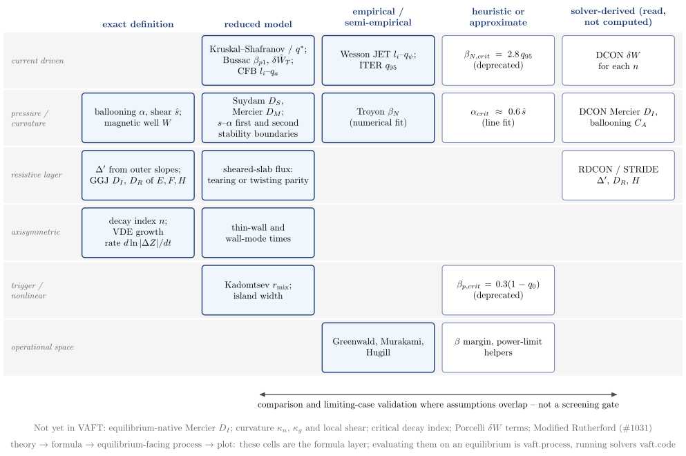
vaft.diagram.stability_diagnostic_taxonomy()
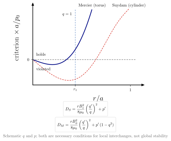
vaft.diagram.interchange_criteria()
 |
 |
| Diagram | Concept |
|---|---|
stability_diagnostic_taxonomy |
VAFT’s criteria by physical problem (rows) and logical status (columns): exact definition, reduced model, empirical or semi-empirical boundary, heuristic, and solver-derived. It also lists what is still absent. The reduced columns are compared with the solvers, not used as a gate |
interchange_criteria |
suydam_criterion and mercier_criterion_circular on one schematic profile. The toroidal $p’(1 - q^2)$ stabilises outside $q = 1$, where Suydam’s criterion still fails |
Single-particle motion
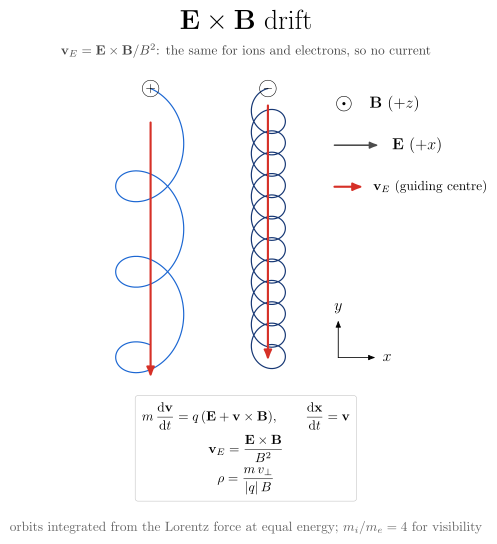
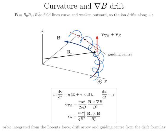
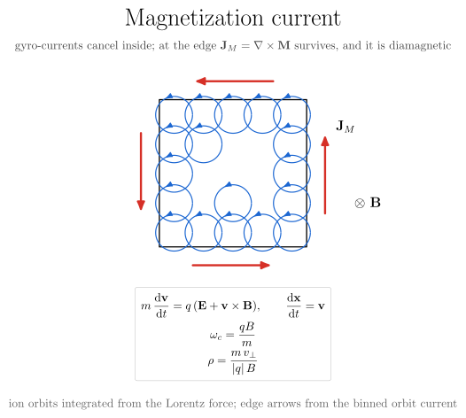
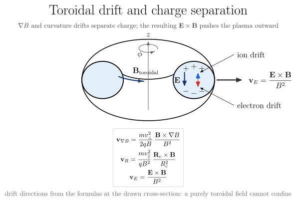
Gyration and guiding-centre drifts, drawn in the island family’s style and 3-D camera. Every orbit
is integrated from the Lorentz force by vaft.formula.boris_orbit, and every drift arrow is the
drift formula of vaft.formula.particle. The tests require the integrated guiding centre to move at
the formula’s velocity, so the figure cannot show a drift that the orbit does not make.
vaft.diagram.exb_drift(mass_ratio=4.0)
vaft.diagram.curvature_drift()
vaft.diagram.magnetization_current()
vaft.diagram.toroidal_drift(aspect_ratio=2.2)
 |
 |
 |
 |
| Diagram | Shows | Arrows from |
|---|---|---|
| E×B drift | An ion and an electron at equal energy in crossed uniform fields. The orbits differ in size, but the drift is the same, so no current flows | exb_drift_velocity |
| Curvature and ∇B drift | An ion spirals along a field line of $B_0R_0/R\,\hat\phi$ and drifts along $+z$ | grad_b_drift_velocity + curvature_drift_velocity |
| Magnetization current | Gyro-currents cancel inside a region. At its edge the diamagnetic $\mathbf{J}_M = \nabla\times\mathbf{M}$ survives | the binned current of the integrated orbits |
| Toroidal drift | ∇B and curvature drifts separate charge. The resulting vertical $\mathbf{E}$ drives an outward $\mathbf{E}\times\mathbf{B}$, so a purely toroidal field cannot confine | the drift formulas at the drawn cross-section |
Every view shows the relevant equations in a box. They are read from the $$…$$ definition in each
formula’s docstring, so the figure shows exactly what the formula documents and implements. There is
no second copy of any equation.
Each has further projections of the same computed orbits, chosen with projection=:
| Diagram | Projections (default first) | What the extra views add |
|---|---|---|
exb_drift |
perpendicular, 3d |
Helices along $\mathbf{B}$ drifting sideways. The parallel velocity does not change the perpendicular motion, so both views show the same orbits |
curvature_drift |
3d, poloidal, top |
poloidal looks along the field line, where the gyration circle climbs at the drift velocity. top shows the curved line and the inward $\nabla B$ |
magnetization_current |
perpendicular, 3d |
Helical columns along $\mathbf{B}$ with the edge current looping around them |
toroidal_drift |
3d, poloidal, top |
poloidal is the textbook $(R, z)$ cross-section. top shows the circular field lines, with the vertical drifts pointing out of the page |
The units are normalised ($|q| = 1$, $m_e = 1$, fields of order one). The ion-to-electron mass ratio is reduced (4 by default) so that both orbits are visible; the figures state this.
Tearing physics
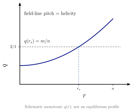
The ideas upstream of an island, one concept per diagram, so each can be used on its own in a page, notebook or slide. None takes an equilibrium, shot or solver output: the curves are schematic.
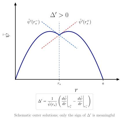
vaft.diagram.rational_surface(m=2, n=1)
vaft.diagram.delta_prime(sign="positive")   # "positive", "zero" or "negative"
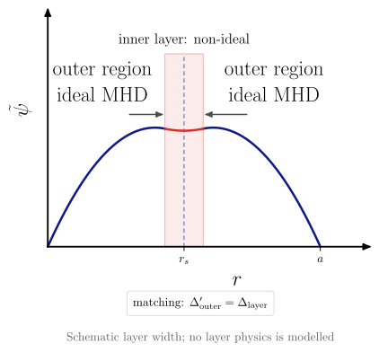
vaft.diagram.tearing_layer_matching()
 |
 |
 |
| Diagram | Question | What is schematic |
|---|---|---|
rational_surface |
Where does a perturbation resonate with the field-line pitch, $q(r_s) = m/n$? | The monotonic $q(r)$; it is not an equilibrium profile |
delta_prime |
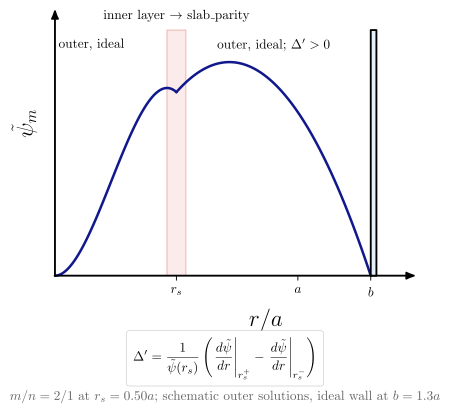
What does the tearing stability index measure? | The outer solutions: quadratics that vanish on the axis and at the edge. Their slopes at $r_s$ go through vaft.formula.delta_prime_from_outer_derivatives, and only the sign of $\Delta’$ is meaningful |
tearing_layer_matching |
Why are the ideal outer regions and the non-ideal inner layer solved separately? | The layer width and the layer solution, which only joins the outer solutions in value and slope |
The index drawn here is the definition, not a stability result: no outer equation is solved. Solver
values of $\Delta’$ (RDCON, STRIDE) belong to vaft.plot, and they are not the RDCON $D_R$ or the
Modified Rutherford terms. The object these lead to is magnetic_island.
3-D perturbation harmonics
How a linear 3-D perturbation is written as complex Fourier harmonics, and what the complex numbers mean. Each diagram is one concept and needs no equilibrium, shot or GPEC output.
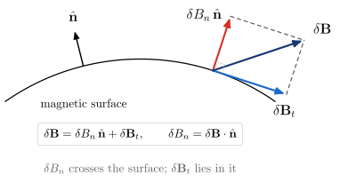
vaft.diagram.normal_field_component()
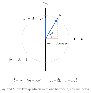
vaft.diagram.complex_harmonic(amplitude=1.0, phase=1.05)
vaft.diagram.toroidal_harmonic_phase(n=1)
vaft.diagram.harmonic_real_space_projection(m=2, n=1, phase=1.05)
vaft.diagram.complex_field_superposition(case="screening")   # "amplification", "phase_shift"
 |
 |
 |
 |
| Diagram | Concept |
|---|---|
normal_field_component |
$\delta B_n = \delta\mathbf B\cdot\hat{\mathbf n}$ is the part of a perturbation that crosses a magnetic surface. It is geometric only, with no code-specific normalisation |
complex_harmonic |
One harmonic is $\hat b = b_R + i\,b_I = A e^{i\alpha}$. $b_R$ and $b_I$ are the cosine and sine quadratures of one pattern, not two fields |
toroidal_harmonic_phase |
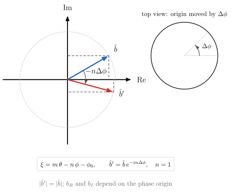
Moving the toroidal origin by $\Delta\phi$ turns $\hat b$ by $-n\Delta\phi$. $\lvert\hat b\rvert$ is invariant; $b_R$ and $b_I$ are not |
harmonic_real_space_projection |
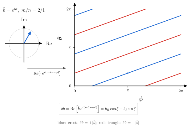
The physical field is real, $\delta b = \mathrm{Re}[\hat b\,e^{i(m\theta - n\phi)}]$ (vaft.formula.helical_harmonic): stripes of slope $n/m$ on the unwrapped $(\phi, \theta)$ plane |
complex_field_superposition |
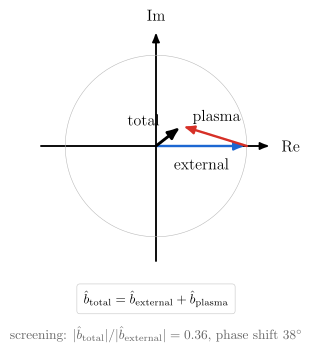
External and plasma-response fields add as complex numbers, so screening, amplification and phase shift all come from one vector sum |
The phase convention is helical_phase’s $\xi = m\theta - n\phi$, with both mode numbers positive and
the helicity in the minus sign. vaft.code.gpec stores each complex quantity as a real/imaginary pair
(i = 0 real, i = 1 imaginary) and rebuilds it as real + 1j * imag, deciding no convention. For
GPEC’s spectral outputs that pair is the $(b_R, b_I)$ of complex_harmonic, and it becomes a field only
through the real-space reconstruction. Two sources differ:
- the
*_funquantities (b_n_fun,xi_n_fun) are already real-space in $\theta$, and GPEC writes them as $(\mathrm{Re}, -h\,\mathrm{Im})$ with its helicity $h$; vaft.process.toroidal_mode_decompositionreturns the conjugate, $\hat b = 2\,\overline{C_n}$.
helical_harmonic’s Convention section states both. Amplitudes, phases and responses in these
figures are schematic.
Collision processes
A classification of the interactions in a fusion plasma, built from the concept-diagram primitives. Coulomb collisions between charged particles relax the distribution. Atomic processes change charge states and bound electrons. Nuclear reactions change nuclei.
vaft.diagram.collision_processes()
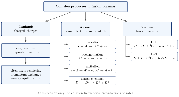
The diagram contains no numbers except the D–T alpha energy, which is vaft.formula.constants.E_ALPHA. Collision frequencies, the
Coulomb logarithm and collisionality regimes are left to formula-backed diagrams (#1111).
Geometric approximations
How slab, cylindrical and toroidal models relate, keeping geometry and ordering on separate axes. The
physics is in vaft.formula.geometry. Geometric approximations
explains each representation.
vaft.diagram.geometry_ordering_map()
vaft.diagram.field_line_geometry(geometry="toroidal")   # "cylindrical", "slab"
vaft.diagram.mode_number_mapping(m=2, n=1)
vaft.diagram.mhd_mode_geometry_map()
| Diagram | Concept |
|---|---|
geometry_ordering_map |
Geometries are columns and orderings are bands. Each reduction arrow names what it keeps or drops |
field_line_geometry |
The same $q$ field line on a torus and on the cylinder straightened at $R_0$, and the tilt of the sheared-slab field lines growing with $x$ |
mode_number_mapping |
The cylinder’s $k_\parallel(r)$ crosses zero at $q(r_s) = m/n$. The local slab of local_slab_from_cylinder is its tangent there |
mhd_mode_geometry_map |
Pressure-driven, current-driven, resonant and $n = 0$ mode families in slab, cylinder and torus. Exact relabelling, limits, analogues and branches are drawn as four different arrows. The text is MHD mode representations across geometries |
Asymptotic orderings
The scale separations a reduced model assumes, evaluated rather than assumed. The kernels are in
vaft.formula.ordering, and Asymptotic orderings (#1627)
explains them. Which diagrams the scale-to-model chain needs, and which are still planned, is
Characteristic scales and orderings, “Diagram contracts”.
vaft.diagram.timescale_hierarchy()
vaft.diagram.spatial_scale_orderings()
vaft.diagram.ordering_contract_map()
vaft.diagram.adapter_contract_map()
| Diagram | Concept |
|---|---|
timescale_hierarchy |
Inverse gyrofrequencies, collision, Alfvén, sound-crossing, inverse ion transit and bounce frequencies, evolution, wall, pulse and resistive times of one illustrative state on one logarithmic axis, each from a formula kernel. Below it are the ordering ratios: $S$, $\tau_{evol}/\tau_A$, $\tau_{pulse}/\tau_R$, $d_i/a$. Drift precession (no kernel) and $\tau_E$ (no inventory) are left out |
spatial_scale_orderings |
Electron and ion Larmor radii, $\rho_s$, $d_i$, the banana width, an illustrative gradient length, $a$, $R_0$ and $qR_0$ of the same state on one logarithmic axis. Below it are $\rho_i/L$, $\Delta_b/L$, $d_i/a$, with brackets for the ratios that need a mode ($k_\perp\rho$, $k_\parallel/k_\perp$, $\omega/\Omega_c$) |
ordering_contract_map |
Which model needs which ordering, read from vaft.validation.orderings.CONTRACTS. Quantities are grouped by scale (foundational, global, profile, perturbation, inner layer, time history) and models by family (fluid, reduced MHD, kinetic, neoclassical, evolution). Each cell is a separate assumption with its own margin, and an empty cell is not ordered. |
adapter_contract_map |
Which ordering contracts each VAFT code-adapter mode consumes, and how each enters the calculation: governing (filled), RDCON’s outer solution and layer solution, DCON-kinetic’s fluid part and kinetic part, PENTRC’s closure, inherited by a reduced model that does not solve its parent theory (dashed). An empty cell is no registered contract, not physical independence (vaft.validation.model_contracts, #1823) |
Plasma-model guide
Figures for the plasma-model guide (#1739). Every node is
read from the formalism records: a node lists the adapter:mode ids of vaft.validation.model_contracts.ADAPTER_MODES
whose record matches it, and codes not in VAFT (vaft.diagram.EXTERNAL_CODES) are hollow and labelled so. Four edge
kinds are used: asymptotic reduction (solid), model coupling (double-headed), software dependency (dotted) and
surrogate ancestry (dashed). No direction is a fidelity axis.
vaft.diagram.plasma_model_reduction_map()
vaft.diagram.formalism_axes_map()
vaft.diagram.solver_placement_map()
vaft.diagram.kinetic_mhd_coupling()
vaft.diagram.reduced_model_ancestry()
| Diagram | Concept |
|---|---|
plasma_model_reduction_map |
One starting point (Vlasov / Fokker–Planck + Maxwell, no VAFT solver) and the reductions to the fluid, drift-kinetic, gyrokinetic, particle, hybrid, reduced and equilibrium descriptions, each edge labelled with its ordering, each node with its VAFT modes |
formalism_axes_map |
The independent axes of vaft.code.formalism.AXES, one column each with an N/A cell, and three runs (CGYRO nonlinear, DCON kinetic, NUBEAM) drawn across them. The numerical representation is a separate box, not an axis |
solver_placement_map |
Every adapter mode against bulk, model, spatial domain and regime, filled from its record, unclassified modes greyed; then the codes not in VAFT, hollow |
kinetic_mhd_coupling |
Kinetic-MHD as a coupling loop between an ideal-MHD bulk and a drift-kinetic population: energy closes it (DCON, GPEC kinetic), closure is one-way (PENTRC), and RDCON’s T_e, n_e input is a coefficient, not a coupling |
reduced_model_ancestry |
Parent theory, model reduction and VAFT realization of every reduced mode; TGLF-NN descends from TGLF. Every row inherits its parent’s contract and adds a closure no contract covers |
Reduced representations
How formulas compress plasma information, from fields to profiles to scalars and from dimensional to
dimensionless quantities, is classified on
Reduced representations (#1626). The figures
are built from the formulas’ Reduction docstring sections and the relation metadata in
vaft.formula._taxonomy.
vaft.diagram.reduced_representation_hierarchy()
vaft.diagram.reduced_representation_hierarchy_compact()
vaft.diagram.reduction_graph(family="current_q")   # "pressure_energy", "kinetic_profiles", "dimensionless_similarity"
| Diagram | Concept |
|---|---|
reduced_representation_hierarchy |
Spatial reduction (field, profile, scalar) down, dimensionless normalisation across, so a dimensionless quantity can still be a profile. Each cell counts the catalogued formulas that land there |
reduced_representation_hierarchy_compact |
The same axes and arrows with only the example symbols in each box, without the counts, at reduced box height and spacing, for slides and overview pages |
reduction_graph |
One family as a layered graph of quantities. A solid edge is a formula, and its catalogued reduction kind is shown as via. A dashed edge is a step VAFT performs elsewhere |
Tokamak geometry and flux coordinates
The parent geometry that the cylindrical and slab reductions start from. Surfaces are
miller_surface, the shift is shafranov_shift_from_r_a_R0_beta_p_li, the field is
vacuum_toroidal_field, and $\theta^*$ is straight_field_line_angle.
vaft.diagram.tokamak_torus(projection="3d")        # "poloidal"
vaft.diagram.flux_surfaces(shape="circular")       # "shifted"
vaft.diagram.shaping_family()
vaft.diagram.hfs_lfs_field()
vaft.diagram.safety_factor_winding(q=3)
vaft.diagram.flux_coordinates()
vaft.diagram.poloidal_angle_comparison()
vaft.diagram.unwrapped_flux_surface(q=2.5)
vaft.diagram.field_line_pitch(q=1.0)
 |
 |
 |
 |
 |
 |
 |
 |
| Diagram | Concept |
|---|---|
tokamak_torus |
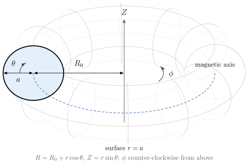
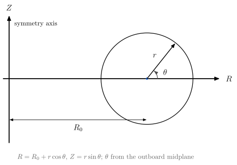
$R_0$, $a$, $\phi$ (counter-clockwise from above) and $\theta$ (from the outboard midplane), with $R = R_0 + r\cos\theta$ |
flux_surfaces |
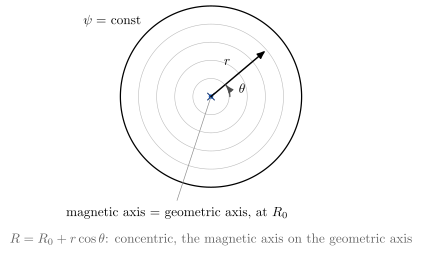
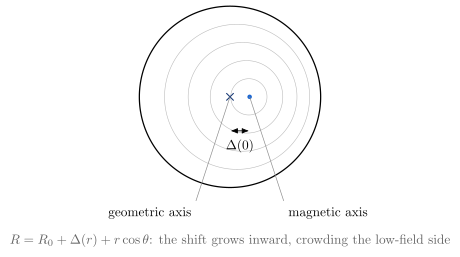
Concentric surfaces, then the Shafranov shift: $\Delta(r)$ is zero at the edge and largest on axis, so the magnetic axis sits outside the geometric axis |
shaping_family |
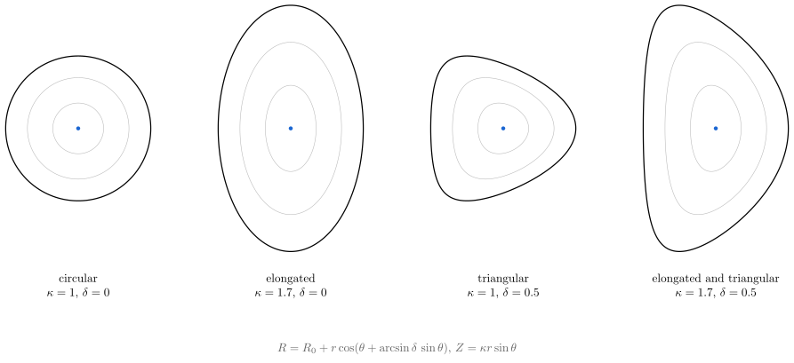
Circular, $\kappa$, $\delta$, and both. Positive triangularity pulls the top in to $R_0 - \delta r$ |
hfs_lfs_field |
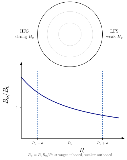
$B_\phi = B_0R_0/R$ is stronger on the inboard (high-field) side |
field_line_pitch |
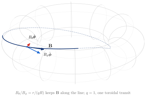
$\mathbf B = B_\phi\hat{\boldsymbol\phi} + B_\theta\hat{\boldsymbol\theta}$ at a point of a field line, with $B_\theta/B_\phi = r/(qR)$ so that $\mathbf B$ lies along the line |
safety_factor_winding |
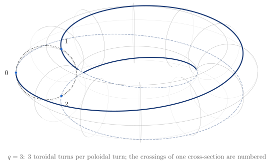
$q$ toroidal turns per poloidal turn, counted at one cross-section |
flux_coordinates |
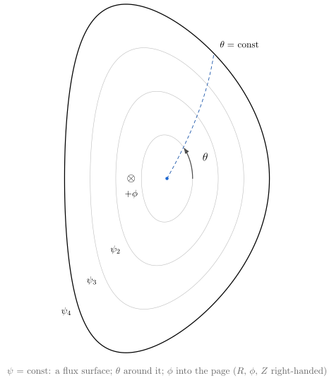
$(\psi, \theta, \phi)$, with $+\phi$ into the page when $R$ is to the right and $Z$ is up |
poloidal_angle_comparison |
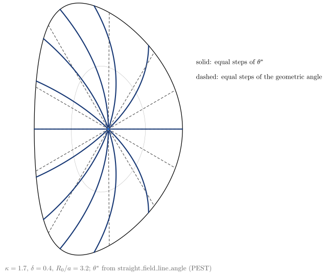
On a D shape, equal steps of $\theta^*$ are not rays of the geometric angle |
unwrapped_flux_surface |
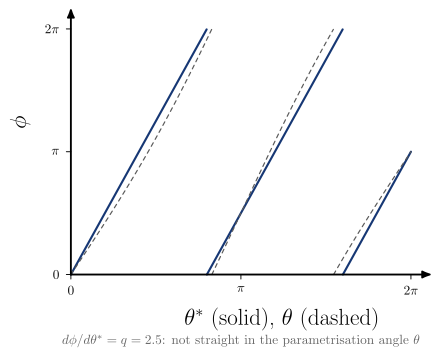
A field line is straight, $d\phi/d\theta^* = q$, in straight-field-line coordinates, and not in the parametrisation angle $\theta$ |
The field line on a torus, its cylindrical and slab reductions, and the geometry/ordering map are in
the geometric-approximations section above. The toroidal → cylindrical → slab bridge is
geometry_ordering_map together with field_line_geometry.
Toroidicity and TF ripple
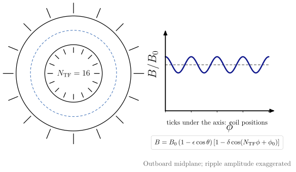
From the $1/R$ mirror to ripple-induced fast-particle transport. The formulas are in
vaft.formula.ripple, and each one names its diagram
under See Also. $B_\phi \propto 1/R$ itself is hfs_lfs_field, in the tokamak-geometry section.
vaft.diagram.trapped_and_passing_orbits()
vaft.diagram.toroidal_field_ripple(n_tf=16)
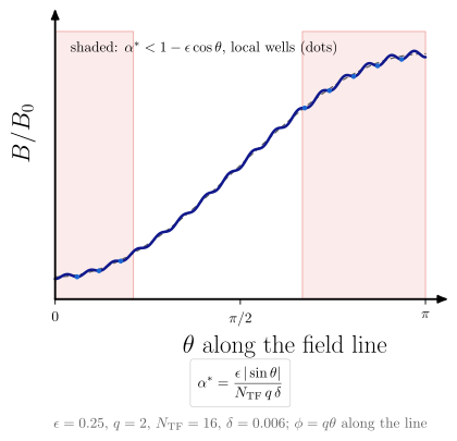
vaft.diagram.ripple_well_formation()
vaft.diagram.stochastic_ripple_orbit()
 |
 |
 |
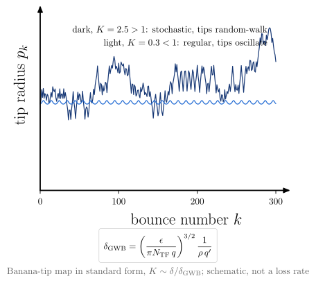 |
| Diagram | Concept | Formula |
|---|---|---|
trapped_and_passing_orbits |
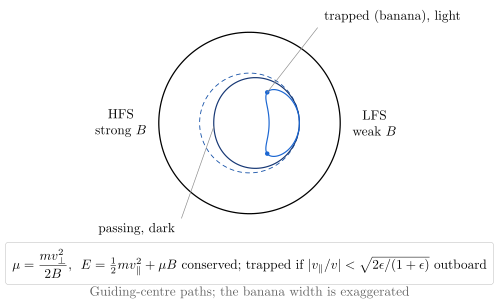
$\mu$ and energy conservation in $B \propto 1/R$: small pitches bounce as bananas, large ones pass | parallel_speed_from_mu, vacuum_toroidal_field |
toroidal_field_ripple |
$N_\mathrm{TF}$ coils corrugate $B(\phi)$: maximal under a coil, minimal between | toroidal_ripple_field, ripple_amplitude |
ripple_well_formation |
Along a field line the ripple makes local wells where $\alpha^* \lesssim 1$, near the midplanes (to first order in $\epsilon$) | ripple_well_parameter |
stochastic_ripple_orbit |
Ripple kicks at banana tips decorrelate above $\delta_\mathrm{GWB}$. Drawn as the standard map with $K \sim \delta/\delta_\mathrm{GWB}$ | gwb_stochastic_threshold, gwb_stochasticity_parameter |
These are regime indicators, not a loss calculation. Orbit following (ASCOT, NUBEAM) is the quantitative check. Low-$n$ error fields, NTV and locking are separate topics.
Guiding-centre invariants and toroidal symmetry
This is the global view of the orbit physics that curvature_drift and toroidal_drift show locally.
The grad-B and curvature drifts say why a guiding centre moves at each instant. Conservation of
$P_\phi$ constrains the whole orbit in an axisymmetric field. These are the same physics seen two
ways, not competing explanations.
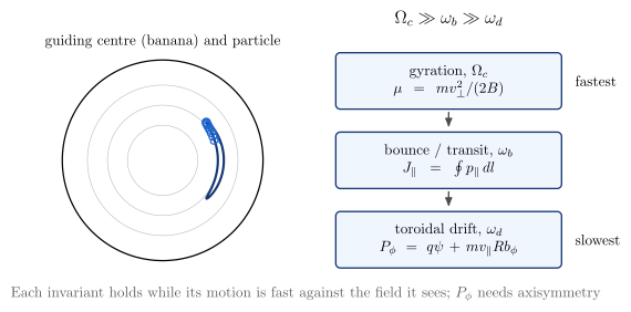
vaft.diagram.guiding_center_invariants()
vaft.diagram.canonical_toroidal_momentum(phase=0.45)
vaft.diagram.toroidal_symmetry_breaking()
 |
 |
| Diagram | Concept | Formula |
|---|---|---|
guiding_center_invariants |
Gyration, bounce and toroidal drift, with invariants $\mu$, $J_\parallel = \oint p_\parallel\,dl$ and $P_\phi$, valid for $\Omega_c \gg \omega_b \gg \omega_d$ | magnetic_moment |
canonical_toroidal_momentum |
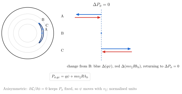
A banana built from $\mu$ and $P_\phi$ conservation. From the bounce tip, $\Delta(q\psi)$ and $\Delta(mv_\parallel Rb_\phi)$ cancel, so $\psi$ moves with $v_\parallel$: this is the orbit width. phase is the state a future animation steps |
guiding_center_toroidal_momentum, parallel_speed_from_mu |
toroidal_symmetry_breaking |
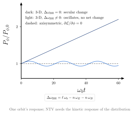
A 3-D field changes $P_\phi$. Away from resonance the change oscillates; where $\Delta\omega_\mathrm{BH} = 0$ it is secular | bounce_harmonic_detuning |
Conventions.
- $P_\phi = mRv_\phi + qRA_\phi$ (
canonical_toroidal_momentum) uses physical components and the IMAS $\phi$. - The guiding-centre form uses $\psi = RA_\phi$ in Wb per radian, largest on the axis for a current
along $+\phi$.
psi_per_radian_from_cocosconverts a stored flux: $-\psi/2\pi$ for COCOS 11 (IMAS DD3) and $+\psi/2\pi$ for COCOS 17 (DD4). Used as stored, the flux has the wrong sign or a $2\pi$ error. - $J_\parallel$ is documented but deliberately not a numerical helper: its bounce interval and orientation depend on the orbit.
- The drift of one orbit’s $P_\phi$ is not NTV. Torque and transport are #1111’s, and need the kinetic response of the whole distribution.
Straight-field-line coordinates
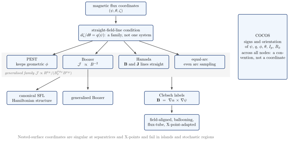
Straight field lines are a condition, not a coordinate system. The freedom the condition leaves is what
PEST, Boozer, Hamada and equal-arc fix in different ways. All four are members of one generalised
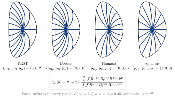
family, $\mathcal{J} \propto R^{p_R}/(B_p^{p_{Bp}}B^{p_B})$ (vaft.formula.generalized_straight_field_line_angle,
as in DCON/GPEC). The unwrapped picture of a straight field line is unwrapped_flux_surface.
Clebsch, field-aligned and ballooning coordinates are #1075’s.
vaft.diagram.sfl_coordinate_grids()
vaft.diagram.sfl_coordinate_taxonomy()
vaft.diagram.sfl_fourier_convergence()
 |
 |
| Coordinate | $(p_{Bp}, p_B, p_R)$ | Geometric $\phi$ kept | Also simplified | Typical use |
|---|---|---|---|---|
| PEST | $(0, 0, 2)$ | yes | the toroidal angle | classical MHD stability |
| Boozer | $(0, 2, 0)$ | no ($\zeta = \phi + \nu$) | $\mathcal{J} \propto B^{-2}$, the $B$ spectrum | orbits, neoclassical, 3-D |
| Hamada | $(0, 0, 0)$ | no | flux-function Jacobian; current lines straight too | MHD stability |
| equal-arc | $(1, 0, 0)$ | no ($\zeta = \phi + \nu$) | uniform poloidal sampling | numerical representation |
- Same equilibrium, different grids. All four panels of
sfl_coordinate_gridsshare one equilibrium: $R_0/a = 1.7$, $\kappa = 2$, $\delta = 0.45$. The surfaces are identical and only the angle changes. A test checks this. - Different Fourier costs. In
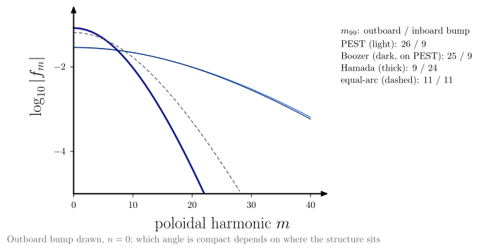
sfl_fourier_convergence, one outboard-localised, axisymmetric perturbation needs anywhere from 9 to 26 poloidal harmonics, depending on the angle it is expanded in. Moved inboard, the ranking reverses: which angle is compact depends on where the structure sits. For $n \ne 0$, the toroidal shift $\nu$ of every angle except PEST couples harmonics further. The figure leaves that out. - Only PEST keeps $\phi$. Keeping the geometric $\phi$ forces $\mathcal{J} \propto R^2$, so every other member has $\zeta = \phi + \nu$.
- Boozer ≈ PEST here. The two nearly coincide at this $B_p \ll B_\phi$, where $B^2 \propto R^{-2}$.
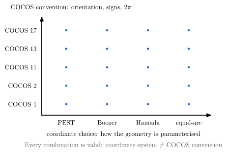
- COCOS is not a coordinate choice. It fixes signs and orientations across every node of the taxonomy, independently of which angle is chosen.
Toroidal shift, action angles, validity, and COCOS
Every straight-field-line angle except PEST needs its own toroidal angle $\zeta = \phi + \nu$.
vaft.formula.equilibrium.sfl_toroidal_angle_shift gives the shift as $\nu = q(\theta_\mathrm{sfl} -
\theta_\mathrm{PEST})$, which follows from $d\phi = q\,d\theta_\mathrm{PEST}$ and $d\zeta = q\,d\theta_\mathrm{sfl}$
along a field line. For a toroidal mode number $n \neq 0$, a mode aligned with the nearest rational surface
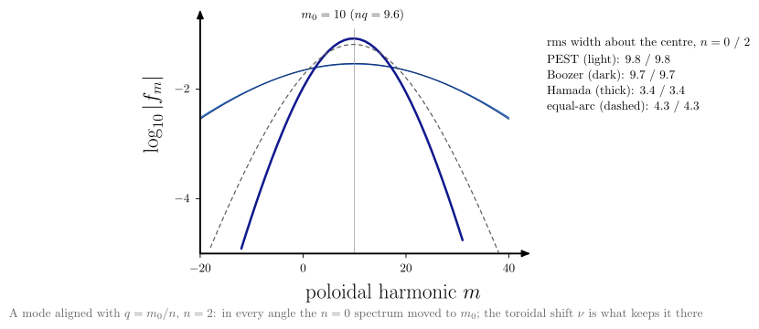
$q = m_0/n$, read at fixed $\zeta$, has in every angle the $n = 0$ spectrum moved to $m \approx m_0$ with its width
unchanged. sfl_fourier_convergence(n=2) shows this: the shift $\nu$ is what keeps such a mode compact. A
structure fixed in the geometric $\phi$ is instead moved by the angle-dependent $\nu$, and stays unshifted only
in PEST (spectra_with_toroidal_mode).
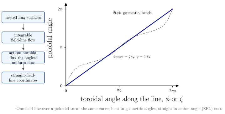
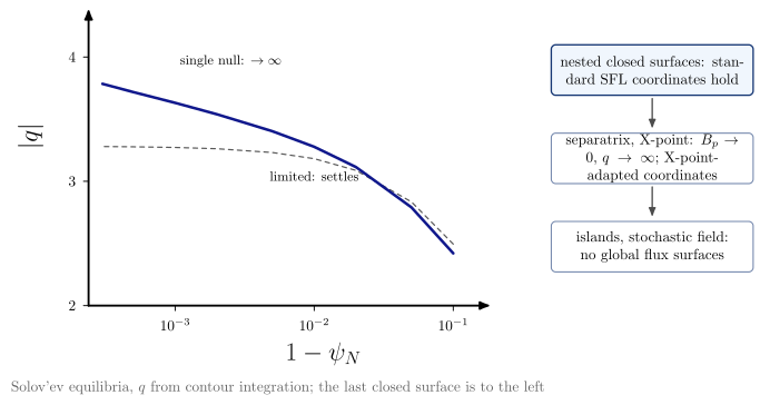
field_line_action_anglefollows one field line over a poloidal turn. Against the geometric angles $(\phi, \vartheta)$ it bends; against $(\zeta, \theta_\mathrm{PEST})$ it is the straight line of slope $1/q$. Nested surfaces make the field-line flow integrable, so SFL coordinates are its action-angle variables; the action is the toroidal flux, and the poloidal flux is the Hamiltonian. Canonical SFL coordinates, which also give the guiding-centre Hamiltonian its canonical form, stay a branch ofsfl_coordinate_taxonomy; no transformation is implemented here.sfl_coordinate_validitycomputes $|q|$ toward the last closed surface. On a limited Solov’ev equilibrium it settles; on a single-null one it grows as $-\ln(1 - \psi_N)$, because $B_p \to 0$ at the X-point and $\theta^*$ degenerates there. Islands and stochastic fields have no global surfaces at all (seemagnetic_islandandstochastic_layer).coordinates_vs_cocosdraws the coordinate choice and the COCOS convention as orthogonal axes: every combination is valid, and a coordinate system is not a COCOS convention.
DCON and GPEC use the generalized family (PEST, Boozer, Hamada, equal-arc, and $J \propto R^{p_R}/(B_p^{p_{B_p}}
B^{p_B})$). An input or output handled in VAFT should therefore keep four things together: the coordinate type,
its powers, the Fourier convention $e^{i(m\theta - n\zeta)}$, and where the mapping came from. Two analyses in
different SFL coordinates describe the same equilibrium with different harmonic content. DCON output
already keeps jac_type and the powers (vaft.code.gpec).
vaft.diagram.sfl_fourier_convergence(n=2)
vaft.diagram.field_line_action_angle()
vaft.diagram.sfl_coordinate_validity()
vaft.diagram.coordinates_vs_cocos()
 |
 |
 |
 |
Clebsch labels and the ballooning representation
These figures go from straight-field-line coordinates to the local, field-aligned and ballooning
descriptions that high-$n$ stability and turbulence models use. The formulas are
field_line_label, s_alpha_curvature_drive and s_alpha_ballooning_solution in
vaft.formula.stability, on the circular $s$–$\alpha$ model.
vaft.diagram.clebsch_field_line_label(q=2.5)
vaft.diagram.ballooning_curvature_drive()
vaft.diagram.ballooning_newcomb_test()
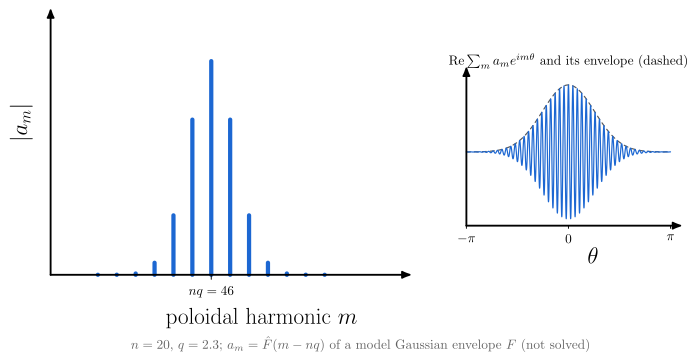
vaft.diagram.ballooning_harmonic_envelope(n=20)
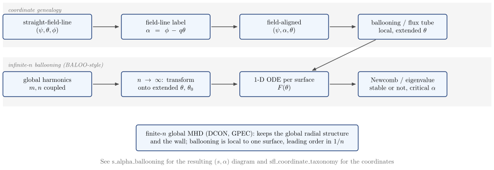
vaft.diagram.ballooning_workflow()
 |
 |
 |
 |
| Diagram | Concept |
|---|---|
clebsch_field_line_label |
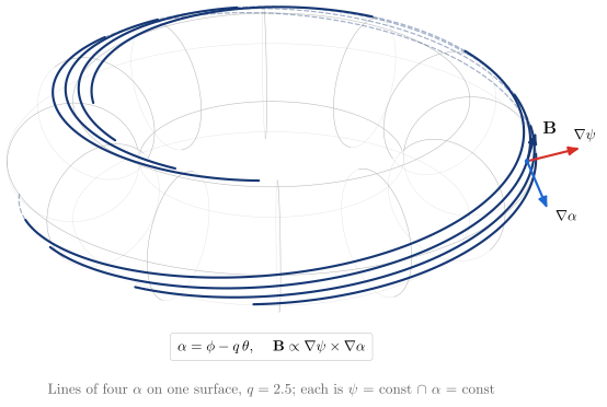
A field line is where $\psi$ = const meets $\alpha = \phi - q\theta$ = const. In helical_phase’s left-handed $(\psi, \theta, \phi)$, with $\psi$ rising outward and $\mathbf B$ along $+\phi$, $\mathbf B \propto \nabla\psi\times\nabla\alpha$. Right-handed coordinates give the Connor–Hastie–Taylor form $\nabla\alpha\times\nabla\psi$ |
ballooning_curvature_drive |
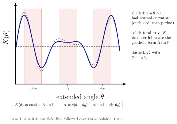
Normal curvature $\cos\theta > 0$ (bad, outboard, shaded) once per $2\pi$ period of the covering space, and the total drive $K = \cos\theta + \Lambda\sin\theta$. Its outer lobes come from the geodesic term, which grows with the local shear. Also shown with $\theta_0$ |
ballooning_newcomb_test |
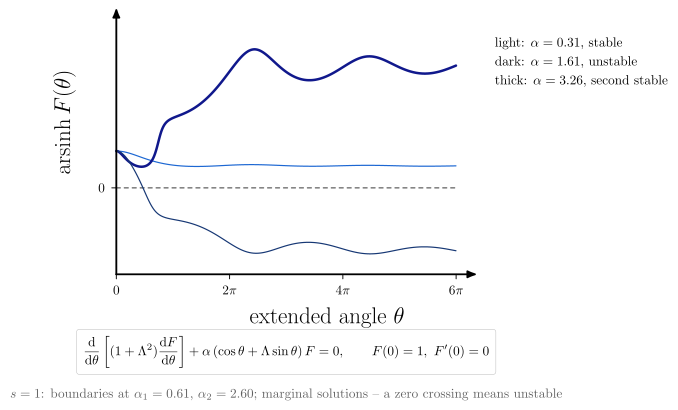
Newcomb’s test on the marginal solution $F(\theta)$: it stays positive (stable), crosses zero (unstable), or is positive again beyond $\alpha_2$ (second stability). These are not localised eigenfunctions |
ballooning_harmonic_envelope |
$a_m = \hat F(m - nq)$ for a stated model envelope: many coupled harmonics around $nq$. Their sum oscillates at $m \approx nq$ under the envelope, localised outboard |
ballooning_workflow |
Straight-field-line coordinates → field-line label → field-aligned → ballooning / flux tube, and the infinite-$n$ path. A finite-$n$ global calculation keeps what that path drops |
The straight-field-line coordinates they start from are in the section above (sfl_coordinate_taxonomy).
The resulting $(s, \alpha)$ stability diagram is s_alpha_ballooning.
Field-aligned basis, flux tube, shear, and the ballooning eigenfunction
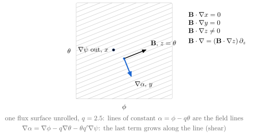
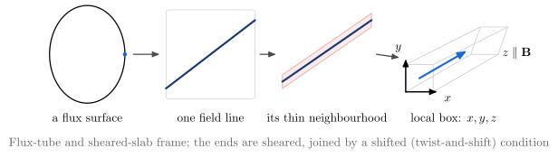
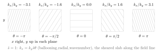
field_aligned_basisunrolls one flux surface. Its field lines are the lines of constant $\alpha = \phi - q\theta$. With $x = \psi$, $y = \alpha$ and $z = \theta$, two coordinates are constant along $\mathbf B$, so $\mathbf B\cdot\nabla = (\mathbf B\cdot\nabla z)\,\partial_z$.flux_tube_patchgoes from a flux surface to one field line, then to its thin neighbourhood, then to the local $(x, y, z)$ box used by flux-tube gyrokinetic codes and by the sheared slab.magnetic_shear_field_alignedfollows a mode along the line. With $k_x = k_y\hat s\theta$ (ballooning_radial_wavenumberat $\alpha = 0$, the $\Lambda$ of the $s$-$\alpha$ model), its phase fronts rotate: the sheared slab’s $k_x(z) = k_{x0} + k_y\hat s z$, seen in the tokamak. The binormal period stays fixed, so the spacing across the fronts shrinks as $1/\sqrt{1+\hat s^2\theta^2}$; that growth of $k_\perp$ is the $(1+\Lambda^2)$ of line bending and inertia.-
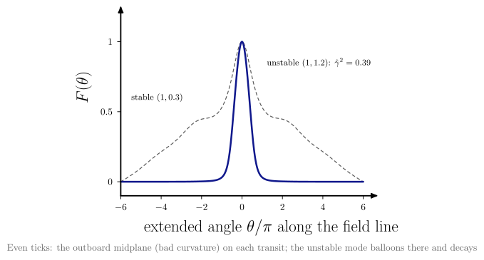
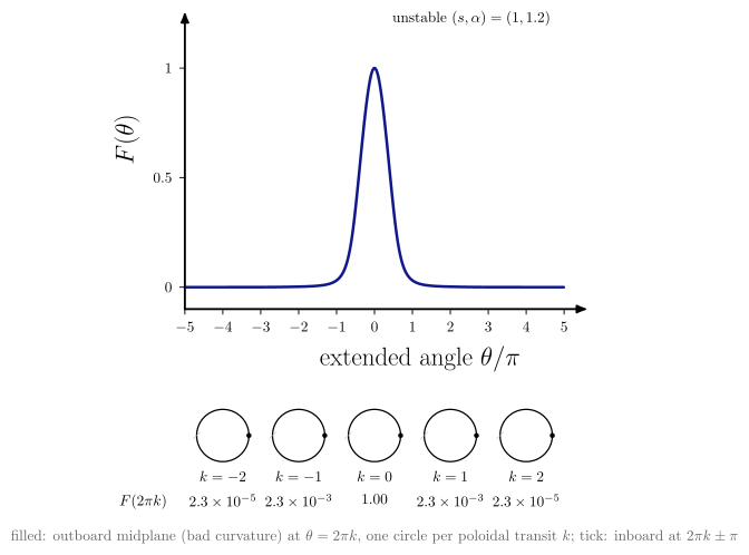
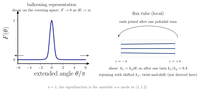
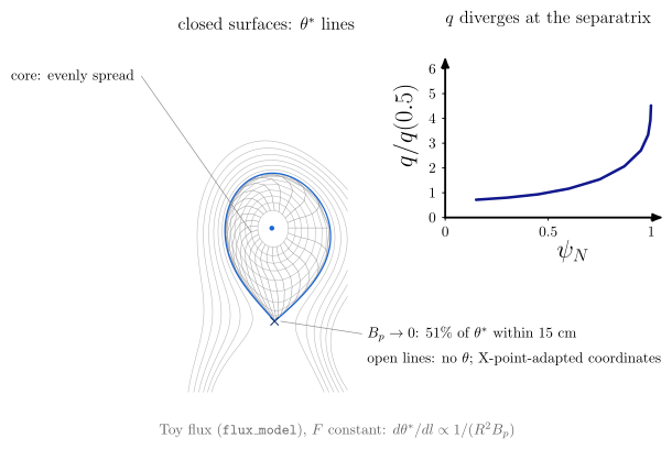
ballooning_eigenfunctionsolves the $s$-$\alpha$ equation with inertia on the extended angle (s_alpha_ballooning_eigenmode). An unstable surface has a mode peaked at the outboard midplane (bad curvature) that decays within a few transits; a stable surface has only the continuum. ballooning_transit_mapties the extended angle to the cross-section: one poloidal circle per transit $k$, under $\theta = 2\pi k$, its outboard point (bad curvature) labelled with $F(2\pi k)$. The same point, revisited on every transit, carries less of the mode each time.ballooning_boundary_conditionsputs the two ways of closing the field line side by side. The ballooning representation requires decay on the covering space, $F \to 0$ as $|\theta| \to \infty$. A flux tube joins its ends after one poloidal turn, and because $k_x = k_y\hat s\theta$ the rejoined end has a shifted $k_x$: twist and shift, named and not derived.field_aligned_xpoint_limitationdraws lines of constant straight-field-line angle $\theta^$ ($d\theta^/dl \propto 1/(R^2B_p)$) on the diverted toy equilibrium of the Grad–Shafranov diagrams. They are evenly spread in the core and crowd into the X-point near the separatrix, where $B_p \to 0$ and $q \propto \oint dl/(R^2B_p)$ diverges; outside it the lines are open and X-point-adapted coordinates take over. See alsosfl_coordinate_validity(#1074).
vaft.diagram.field_aligned_basis(q=2.5)
vaft.diagram.flux_tube_patch()
vaft.diagram.magnetic_shear_field_aligned(shear=1.0)
vaft.diagram.ballooning_eigenfunction()
vaft.diagram.ballooning_transit_map(transits=2)
vaft.diagram.ballooning_boundary_conditions(shear=1.0)
vaft.diagram.field_aligned_xpoint_limitation(n_theta=24)
 |
 |
Ballooning formulations
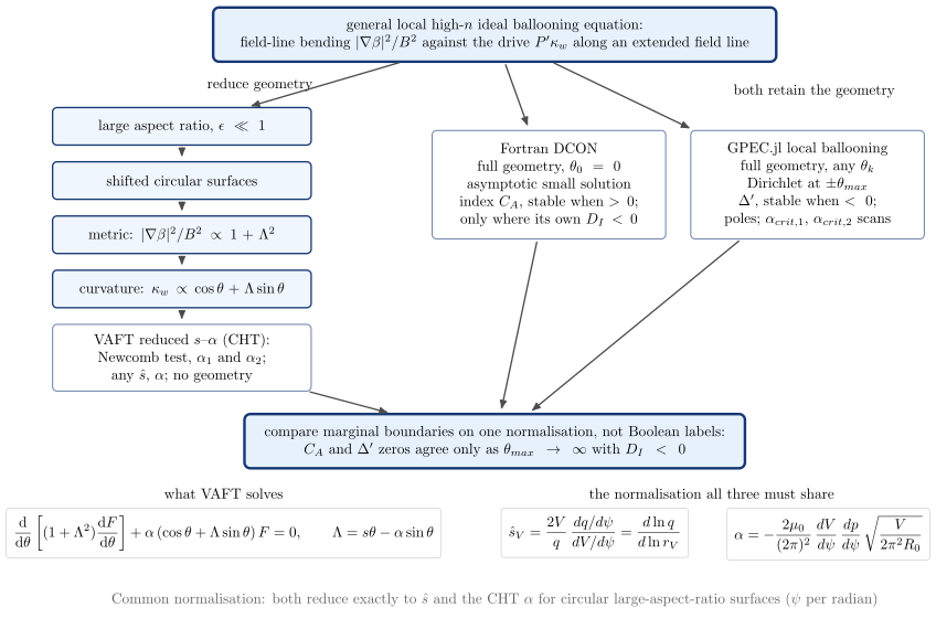
How the reduced $s$–$\alpha$ equation follows from the general ballooning equation, and how DCON’s $C_A$ and GPEC.jl’s ballooning $\Delta’$ relate to it, is on Ballooning formulations (#1637).
vaft.diagram.ballooning_formulation_hierarchy()
| Diagram | Concept |
|---|---|
ballooning_formulation_hierarchy |
The general equation either loses its geometry step by step (large aspect ratio, shifted circles, the $1 + \Lambda^2$ metric, the $\cos\theta + \Lambda\sin\theta$ curvature) to become the CHT equation VAFT solves, or keeps it, as DCON ($C_A$, stable when positive) and GPEC.jl ($\Delta’$, stable when negative, with poles) do. All three must share the normalisation of shear_from_volume and ballooning_alpha_from_volume before their boundaries can be compared |
Slab resonant layers: tearing and twisting parity
How a global harmonic becomes a local layer response. The mapping $(m, n) \to (k_y, k_z)$ and
$q = m/n \Leftrightarrow k_\parallel = 0$ is mode_number_mapping. The flux is
vaft.formula.slab_perturbed_flux; its tearing form is the island pendulum of magnetic_island.
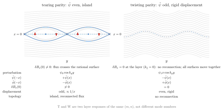
vaft.diagram.slab_parity(parity="tearing")   # "twisting"
vaft.diagram.slab_parity_comparison()
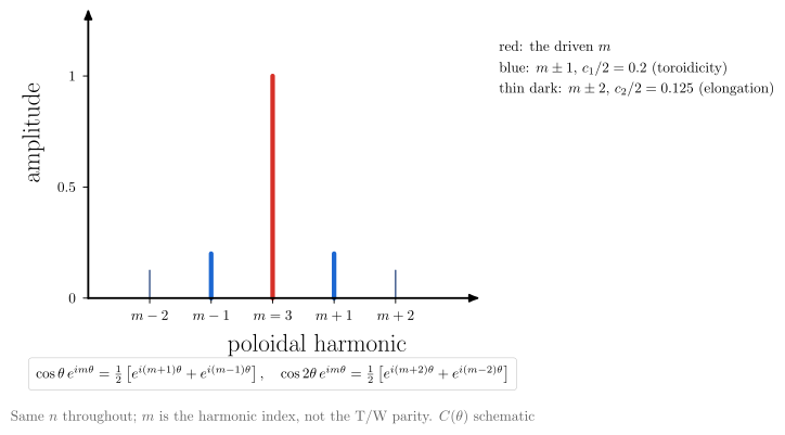
vaft.diagram.poloidal_harmonic_coupling(m=3)
vaft.diagram.resonant_layer_matching()
 |
 |
| Diagram | Concept |
|---|---|
slab_parity |
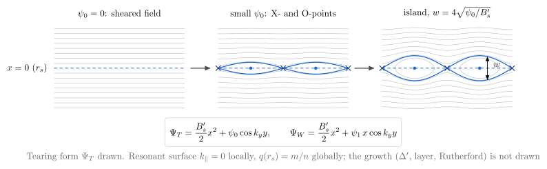
Contours of $\Psi_T = B_s’x^2/2 + \psi_0\cos k_yy$: an island of width $4\sqrt{\psi_0/B_s’}$, O- and X-points, and $\delta B_x(0) \ne 0$. Contours of $\Psi_W = B_s’x^2/2 + \psi_1x\cos k_yy$, drawn with its $O(\psi_1^2)$ completion: no normal field at the layer ($k_\parallel = 0$) and no reconnection, and every surface, the rational one included, displaced together by $\xi = -\psi_1\cos k_yy/B_s’$ |
slab_parity_comparison |
Both side by side, with the parity of $\tilde\psi$ and $\tilde\phi$, $\delta B_x(0)$ and the topology |
poloidal_harmonic_coupling |
$\cos\theta$ (toroidicity) couples $m \to m \pm 1$ and $\cos 2\theta$ (elongation) couples $m \to m \pm 2$, at fixed $n$. The harmonic index $m$ is not the parity |
resonant_layer_matching |
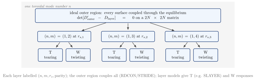
Every rational surface of one $n$ has a T and a W channel. The outer region couples them all into one $2N\times2N$ matrix (RDCON/STRIDE), and each layer is solved on its own (SLAYER) |
Cylindrical geometry: profiles, mode shapes and matching
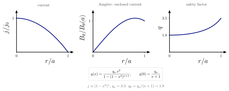
The screw-pinch picture between the torus and the slab. The profile is Wesson’s peaked current
$j \propto (1 - x^2)^\nu$, given by peaked_current_safety_factor together with
cylindrical_poloidal_field (Ampère). The screw-pinch field line is
field_line_geometry("cylindrical"), and the cylinder-versus-torus harmonic contrast is
poloidal_harmonic_coupling.
vaft.diagram.current_to_q_profile(nu=1.0, q_a=3.5)
vaft.diagram.cylindrical_rational_surfaces(n=1)
vaft.diagram.cylindrical_mode_morphology()
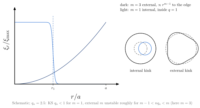
vaft.diagram.internal_external_kink()
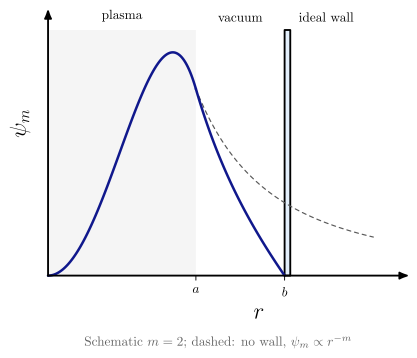
vaft.diagram.plasma_vacuum_wall(m=2)
vaft.diagram.cylindrical_tearing_outer(m=2, n=1)
 |
 |
 |
 |
| Diagram | Concept |
|---|---|
current_to_q_profile |
$j \to B_\theta \to q$. More peaked current means lower $q_0 = q_a/(\nu+1)$ and stronger shear |
cylindrical_rational_surfaces |
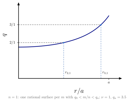
For one $n$, one surface $q(r_s) = m/n$ for each $m$ between $q_0$ and $q_a$ |
cylindrical_mode_morphology |
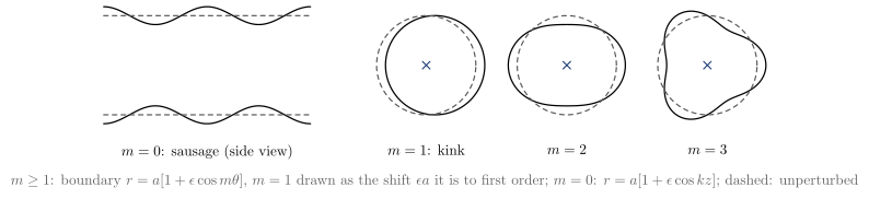
$m = 0$ sausage, $m = 1$ kink (a rigid shift), $m = 2, 3$ helical distortions |
internal_external_kink |
The $m = 1$ internal kink lives inside $q = 1$. An external kink reaches the boundary. Kruskal–Shafranov is a heuristic |
plasma_vacuum_wall |
One harmonic matched across plasma, vacuum ($Ar^m + Br^{-m}$) and an ideal wall |
cylindrical_tearing_outer |
The outer solutions at $r_s$ and their $\Delta’$, for the outer, ideal problem. The inner layer at $r_s$ is slab_parity |
From the cylinder to the slab: mode_number_mapping expands $k_\parallel(r)$ about $r_s$ into the local
slab of local_slab_from_cylinder, and resonant_layer_matching couples several such layers.
The screw-pinch field line itself is field_line_geometry("cylindrical"), and the cylinder-vs-torus harmonic
picture (independent $m$ vs toroidally coupled $m, m\pm1$) is poloidal_harmonic_coupling.
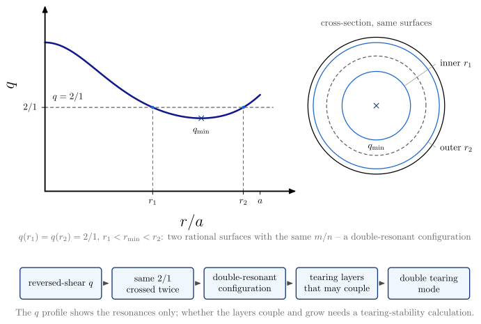
Current-profile and q topology
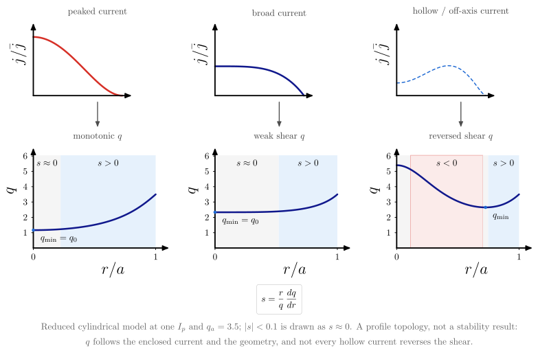
What the shape of the current does to the poloidal field, the internal inductance and the safety
factor, and how the shape of $q$ decides how many rational surfaces one $m/n$ has (#1604). All four
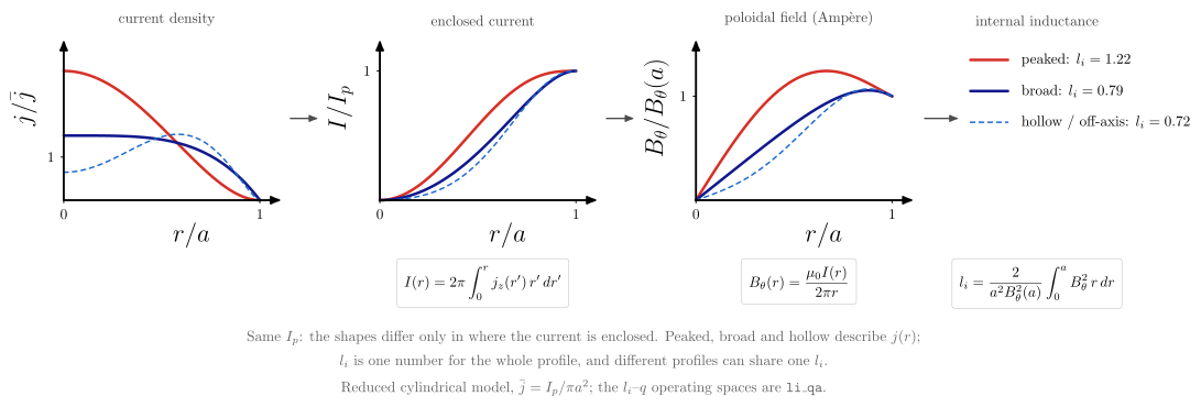
diagrams use one reduced model: a straight cylinder whose current is peaked
($j \propto (1 - x^2)^2$), broad ($1 - x^4$) or hollow / off-axis ($(0.1 + x^2)(1 - x^2)^{3/2}$), each
normalized to the same $I_p$. The chain is cylindrical_enclosed_current, cylindrical_poloidal_field
(Ampère), cylindrical_safety_factor_from_r_B, cylindrical_poloidal_flux (for $\psi_N$),
cylindrical_internal_inductance and shear_from_r_q. The crossings come from
vaft.process.equilibrium.find_rational_surfaces, the routine that finds them on a reconstructed $q$.
These are concept figures, not equilibria and not stability results.
vaft.diagram.current_profile_shapes()
vaft.diagram.q_profile_topologies()
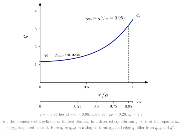
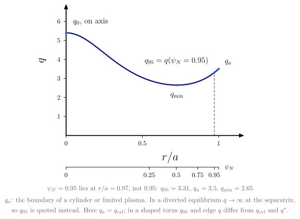
vaft.diagram.q_profile_landmarks(profile="monotonic")         # or "reversed_shear"
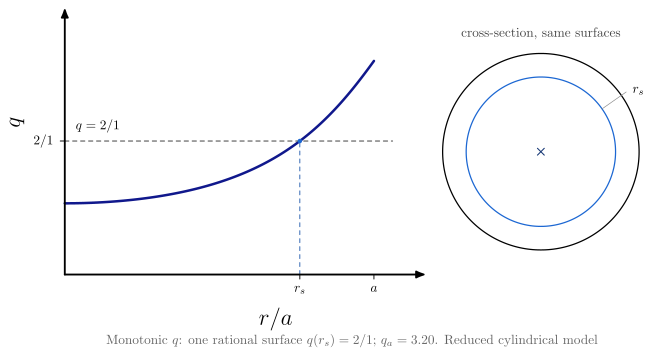
vaft.diagram.rational_surface_topology(profile="reversed_shear", m=2, n=1)
 |
 |
 |
 |
| Diagram | Concept |
|---|---|
current_profile_shapes |
$j(r) \to I(r) \to B_\theta(r) \to l_i$ at fixed $I_p$. Peaked, broad and hollow are shapes of the current density. $l_i$ is one number for the whole profile: a more centrally enclosed current tends to a larger $l_i$, but different profiles can share one $l_i$ |
q_profile_topologies |
Peaked current gives a monotonic $q$, broad current a wide weak-shear core ($s \approx 0$), hollow current a reversed-shear $q$ with $s < 0$ inside $q_{\min}$. Every $q$ has $s \to 0$ on axis, so each column carries a narrow $s \approx 0$ band there; the width of the flat core is the discriminator. Not every hollow current reverses the shear |
q_profile_landmarks |
$q_0$ on axis; $q_{\min}$, equal to $q_0$ only when $q$ is monotonic; $q_{95} = q(\psi_N = 0.95)$, which is not at $r/a = 0.95$; $q_a$, the boundary value of a cylinder or limited plasma. In a diverted equilibrium $q \to \infty$ at the separatrix, so $q_{95}$ is quoted. In the cylinder $q_a = q_\mathrm{cyl}$; in a shaped torus $q_{95}$ and the edge $q$ differ from $q_\mathrm{cyl}$ and $q^*$ |
rational_surface_topology |
A monotonic $q$ crosses one $m/n$ once. A reversed-shear $q$ can cross it twice, $q(r_1) = q(r_2) = m/n$ with $r_1 < r_{\min} < r_2$: a double-resonant configuration. A double tearing mode is the instability in which tearing layers on the two surfaces couple, and only a stability calculation can say whether it grows |
These diagrams sit upstream of the others. current_to_q_profile keeps the analytic peaked
family $j \propto (1 - x^2)^\nu$ and cylindrical_rational_surfaces the monotonic surfaces of one $n$
(#1072). rational_surface keeps the single-crossing definition, and delta_prime and
tearing_layer_matching follow it (#1039). The $l_i$–$q$ diagrams of li_qa (#1603) are
operating spaces: one scalar $l_i$ against one scalar edge $q$, from the literature. They are not
plots of a current profile. The data-side counterparts are vaft.plot.equilibrium_profile_j_tor and
equilibrium_profile_q (#1505).
Current diffusion and current drive
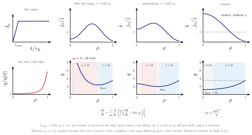
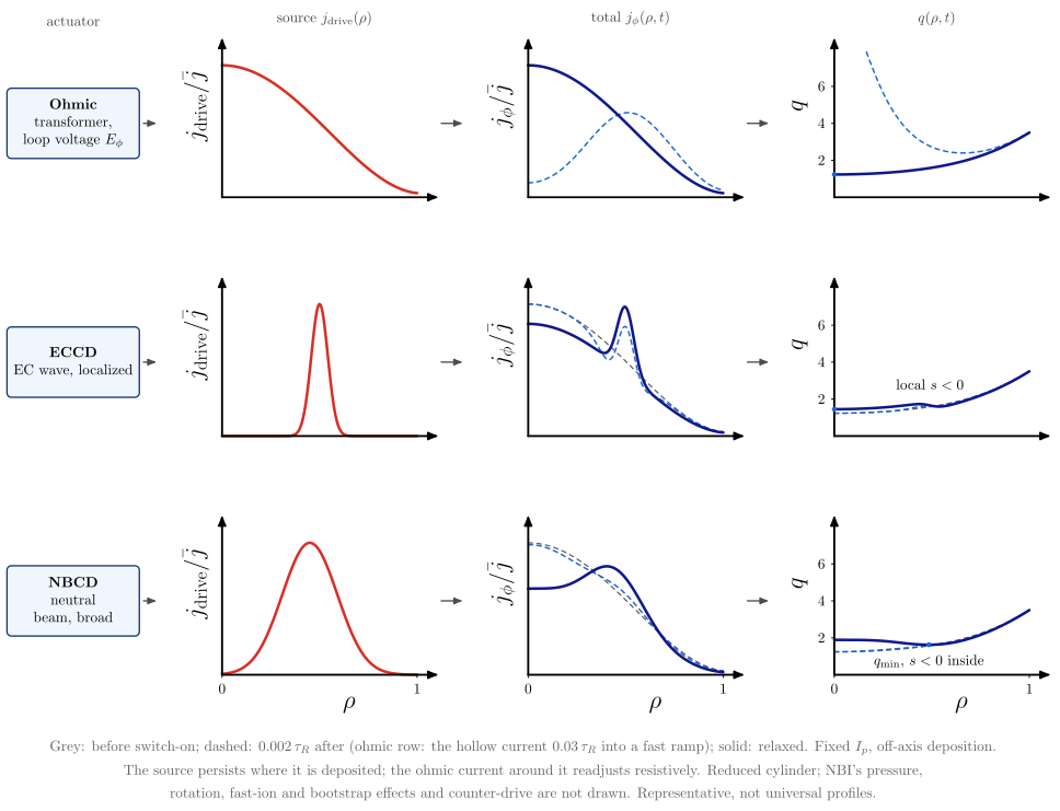
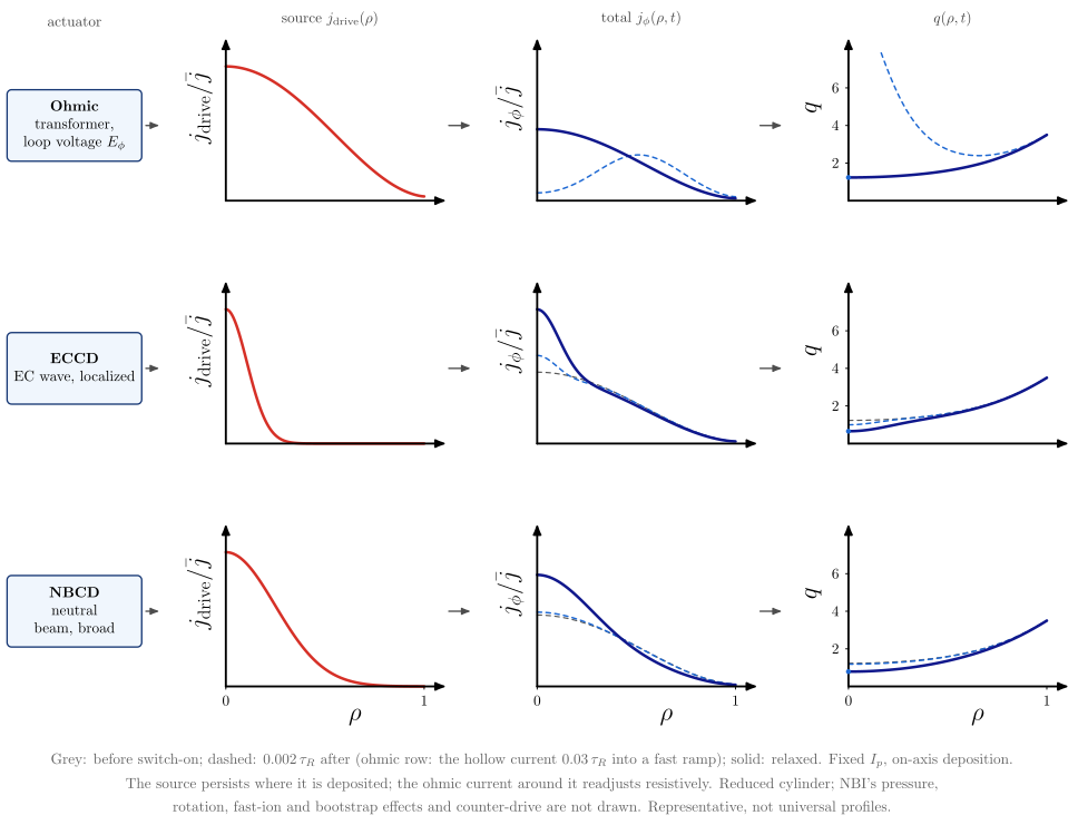
How the current-density and safety-factor profiles above form in time (#1605). Both diagrams evolve one
reduced model: the enclosed current $I(\rho, t)$ of a straight cylinder under
cylindrical_current_diffusion_rate (Faraday, Ampère and Ohm’s law with a non-inductive source
$j_\mathrm{ni}$), integrated implicitly. The resistivity is a fixed Spitzer
$\eta(\rho)$ (spitzer_resistivity_from_T_e_Z_eff_ln_Lambda) on a hot-core, cold-edge $T_e(\rho)$, and
time is in units of the core resistive_diffusion_time $\tau_R = \mu_0 a^2/\eta(0)$. The profiles are
representative, not universal: there is no transport, bootstrap current or toroidal geometry.
vaft.diagram.current_diffusion()
vaft.diagram.current_drive_profiles(deposition="off_axis")   # or "on_axis"
 |
 |
| Diagram | Concept |
|---|---|
current_diffusion |
A fast ohmic ramp, $t_\mathrm{ramp} = 0.01\,\tau_R \ll \tau_R$ (the ordering of a fast ramp such as VEST’s; the ratio is illustrative), leaves the current in an off-axis shell, depleted at the cold edge: hollow $j_\phi$, $q_{\min}$ off axis and $s < 0$ inside it. The current then penetrates and relaxes towards $j_\phi \propto 1/\eta$ with one $E_\phi$ across the radius. The relaxed profile is peaked only because the core is hotter; with a uniform $\eta$ (dashed) the same diffusion relaxes to a flat current |
current_drive_profiles |
Ohmic, ECCD and NBCD rows: actuator, the source $j_\mathrm{drive}(\rho)$ it drives, the total $j_\phi(\rho, t)$ before, shortly after and long after switch-on, and $q(\rho, t)$. The driven source persists where it is deposited while the ohmic current around it readjusts resistively; the source itself does not diffuse. ECCD is narrow and modifies the local shear; NBCD is broad. NBI’s pressure, rotation, fast-ion and bootstrap effects and counter-drive are not drawn |
Field configurations, reconnection and MHD waves
The canonical slab configurations, the topology of reconnection, and the linear ideal-MHD waves.
All are drawn in the slab frame of vaft.formula.geometry: $x$ is the sheet normal (radial), $y$ the
reconnecting (binormal) direction, and $z$ the current and guide-field direction. The geometry itself
(slab, sheared slab, cylinder, torus) belongs to Geometric approximations.
The formulas are harris_sheet_field, harris_sheet_current_density and x_point_flux in geometry,
and shear_alfven_frequency and magnetosonic_phase_speeds in stability.
vaft.diagram.slab_field_configuration(kind="sheared")   # "uniform", "reversed", "guide"
vaft.diagram.current_sheet(guide_field=False)
vaft.diagram.harris_sheet()
vaft.diagram.x_point()
vaft.diagram.magnetic_reconnection()
vaft.diagram.island_formation()
vaft.diagram.shear_alfven_wave()
vaft.diagram.fast_magnetosonic_wave()
vaft.diagram.mhd_wave_family()
 |
 |
 |
 |
 |
 |
 |
 |
| Diagram | Concept |
|---|---|
slab_field_configuration |
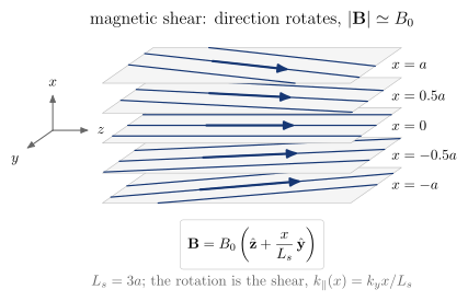
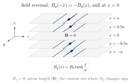
The field on stacked $x$ = const sheets. Uniform; sheared, where the direction rotates and $\lvert\mathbf B\rvert = B_0$ to first order in $x/L_s$; reversed, where $B_y(-x) = -B_y(x)$ with a null at $x = 0$; and reversed with a guide field $B_g$, which rotates with no null. Shear and reversal are different things |
current_sheet |
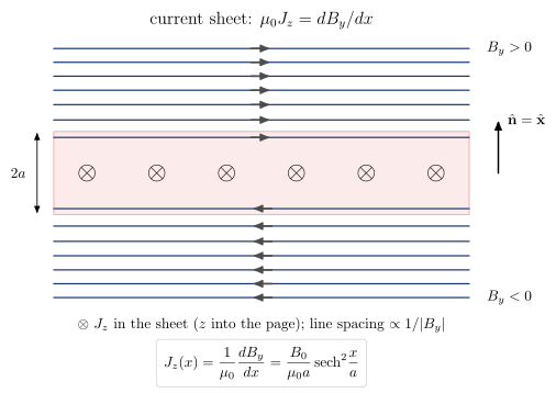
The reversing Harris field seen along the current, with lines at equal flux spacing (spacing $\propto 1/\lvert B_y\rvert$), the sheet of thickness $2a$, its normal, and $\otimes J_z$. With guide_field=True, $B_g\hat{\mathbf z}$ removes the null and leaves $J_z$ unchanged |
harris_sheet |
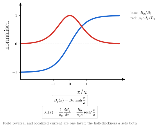
$B_y = B_0\tanh(x/a)$ and $J_z = (B_0/\mu_0a)\,\mathrm{sech}^2(x/a)$ on one chart: the reversal and the localized current are the same layer |
x_point |
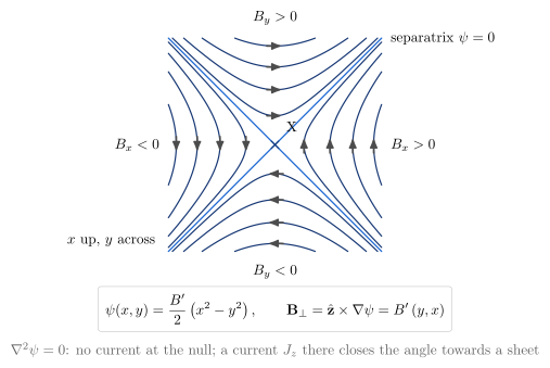
The current-free null $\psi = B’(x^2 - y^2)/2$: four branches and two separatrices at right angles. Geometry only |
magnetic_reconnection |
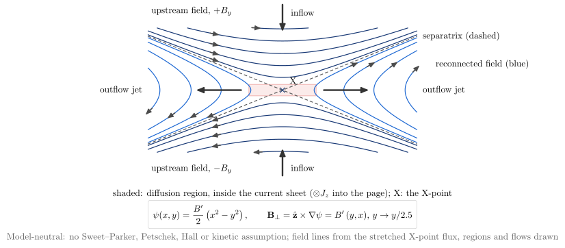
Model-neutral reconnection: inflow, outflow jets, diffusion region, upstream and reconnected field lines about a stretched X-point. No Sweet–Parker, Petschek, Hall or kinetic assumption |
island_formation |
slab_perturbed_flux with growing $\psi_0$: straight sheared lines, then X- and O-points, then an island of width $w = 4\sqrt{\psi_0/B’}$. The growth is delta_prime, slab_parity and tearing_layer_matching |
shear_alfven_wave |
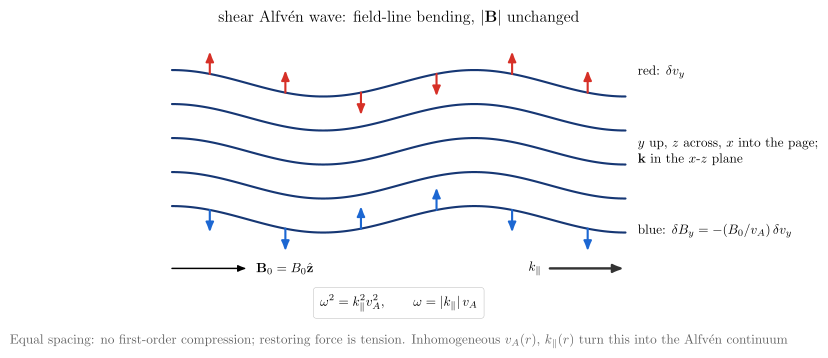
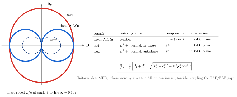
Field-line bending with equally spaced lines, so $\lvert\mathbf B\rvert$ is unchanged to first order. $\delta\mathbf v_\perp$ and $\delta\mathbf B_\perp = -(B_0/v_A)\delta\mathbf v_\perp$ lie normal to the $\mathbf k$-$\mathbf B_0$ plane, and $\omega = \lvert k_\parallel\rvert v_A$ |
fast_magnetosonic_wave |
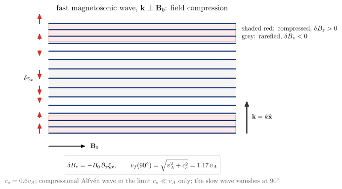
At $\mathbf k \perp \mathbf B_0$ the lines bunch and spread, $\delta B_z = -B_0\partial_x\xi_x$, and $v_f = (v_A^2 + c_s^2)^{1/2}$. It is the compressional Alfvén wave only in the limit $c_s \ll v_A$ |
mhd_wave_family |
The Friedrichs diagram of fast, shear-Alfvén and slow phase speeds against the angle to $\mathbf B_0$ ($v_s \le v_A\lvert\cos\theta\rvert \le v_f$), with each branch’s restoring force, compressibility and polarization |
From these to the tokamak: the current sheet and the island lead to the tearing layer (slab_parity),
then to the cylindrical and toroidal tearing mode (delta_prime, resonant_layer_matching). Here
$q(r_s) = m/n$ globally is $k_\parallel = 0$ locally (mode_number_mapping). The uniform-slab shear
Alfvén wave leads to the Alfvén continuum, where $v_A(r)$ and $k_\parallel(r)$ vary. Toroidal coupling
(poloidal_harmonic_coupling) then opens the gaps of the TAE and EAE. Those are not computed here.
The Grad–Shafranov problem: regions, boundaries and problem classes
The axisymmetric field is $\mathbf B = R^{-1}\nabla\psi\times\hat{\boldsymbol\phi} + F(\psi)R^{-1}\hat{\boldsymbol\phi}$,
with $\psi$ the poloidal flux per radian and $F = RB_\phi$ the poloidal-current function. Its components are
radial_magnetic_field_from_psi and vertical_magnetic_field_from_psi (COCOS-aware); in vacuum $F$ is constant, and
$B_\phi = F/R$ is vacuum_toroidal_field. One flux function $\psi(R, Z)$ is solved across the plasma, vacuum and coil regions, each with its own
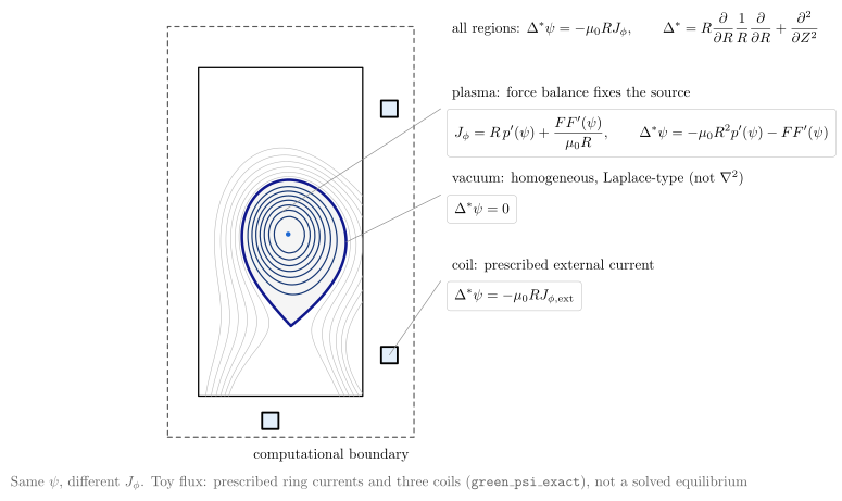
source. vaft.formula.grad_shafranov_source gives the Ampère form $\Delta^*\psi = -\mu_0RJ_\phi$,
which holds in every region. toroidal_current_density_from_p_prime_ff_prime gives the plasma current
that force balance allows, $J_\phi = Rp’ + FF’/(\mu_0R)$. On a grid, the operator is
vaft.process.equilibrium.grad_shafranov_operator. The flux maps are a toy: prescribed ring currents
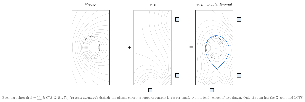
and three coils superposed through green_psi_exact. The topology (axis, X-point, limiter contact, LCFS)
is then found from the total flux, as a free-boundary code finds it. A production solver would also make
the plasma current consistent with $p’$ and $FF’$.
vaft.diagram.grad_shafranov_domain_decomposition()
vaft.diagram.fixed_vs_free_boundary_equilibrium()
vaft.diagram.limiter_and_diverted_topologies()
vaft.diagram.equilibrium_problem_taxonomy()
vaft.diagram.poloidal_flux_source_decomposition()
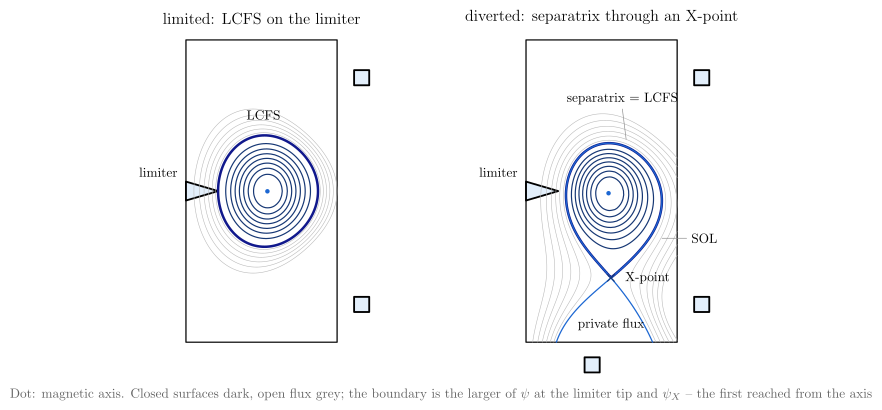
| Diagram | Concept |
|---|---|
grad_shafranov_domain_decomposition |
Same $\psi$, different $J_\phi$. The plasma source comes from force balance. The vacuum is homogeneous, $\Delta^*\psi = 0$: Laplace-type, but not $\nabla^2$. A coil carries its prescribed current. All of this sits inside the computational boundary |
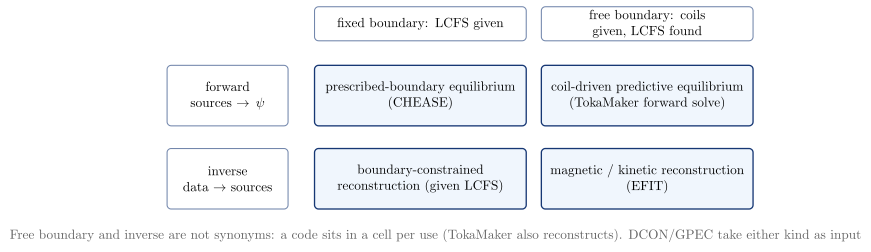
fixed_vs_free_boundary_equilibrium |
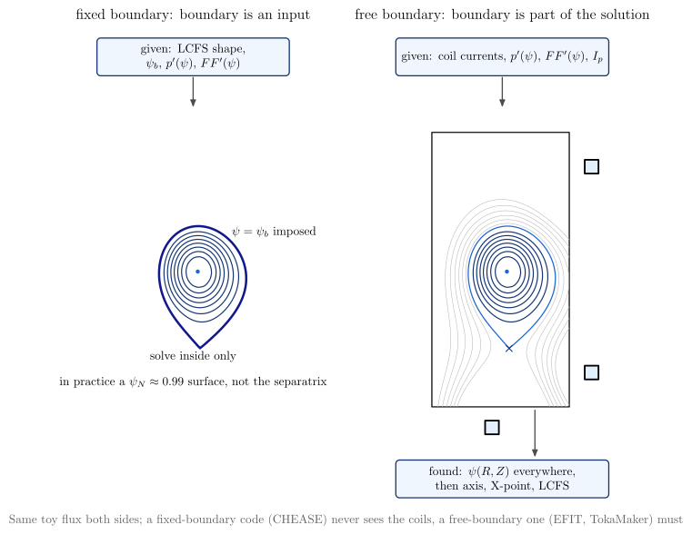
The boundary is an input (LCFS and $\psi_b$ given, only the inside solved) or it is part of the solution (coils and sources given, $\psi$ everywhere, LCFS read from the topology) |
limiter_and_diverted_topologies |
Limited: the LCFS is the surface through the limiter tip. Diverted: the separatrix through the X-point ($\nabla\psi = 0$), with SOL and private flux. The boundary is the larger of $\psi_\mathrm{lim}$ and $\psi_X$ |
equilibrium_problem_taxonomy |
Forward/inverse and fixed/free are separate axes. CHEASE is forward and fixed, TokaMaker forward and free, EFIT inverse and free. Free boundary and inverse are not synonyms |
poloidal_flux_source_decomposition |
$\psi_\mathrm{plasma} + \psi_\mathrm{coil} = \psi_\mathrm{total}$. Only the sum has the X-point and the LCFS. $\psi_\mathrm{passive}$ (eddy currents) is a further term, not drawn |
Equilibrium-aware phenomena: kink displacement and sawtooth
This layer sits between the reference diagrams and result plotting. The geometry comes from an
equilibrium (any vaft.data.equilibrium.EquilibriumData); the physical state is a prescribed, documented
model. The default equilibrium is the exact Solov’ev (Cerfon–Freidberg) equilibrium of
vaft.process.equilibrium.solovev_example with $A = 0$, where $q$ rises from about 0.8 to 3. Surfaces,
normals and the PEST angle $\theta^$ come from straight_field_line_map, and $q(\rho)$ from
calculate_q_profile_from_psi, with $\rho = \sqrt{\psi_N}$. The mode phase uses $\theta^$. The drawing
uses the real $(R, Z)$ surfaces.
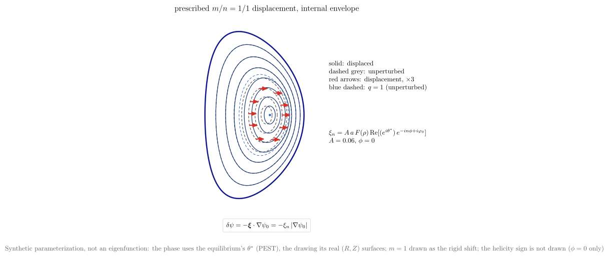
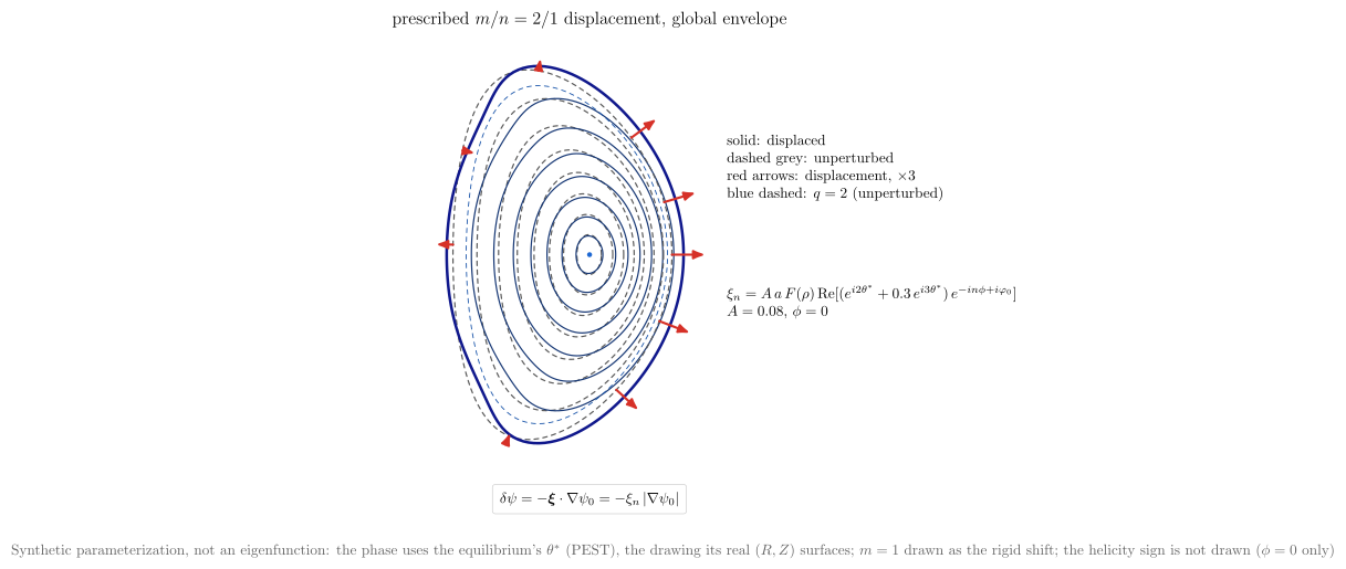
vaft.diagram.kink_mode(equilibrium=None, m=1, n=1, amplitude=0.06, radial_profile="internal")
vaft.diagram.kink_mode(m=2, n=1, radial_profile="global", harmonics={2: 1.0, 3: 0.3})
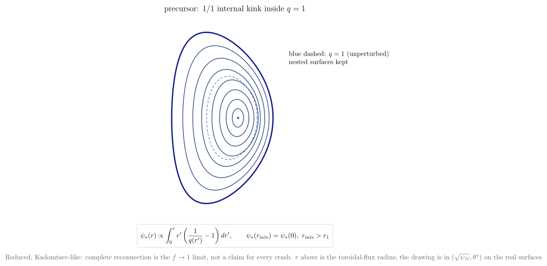
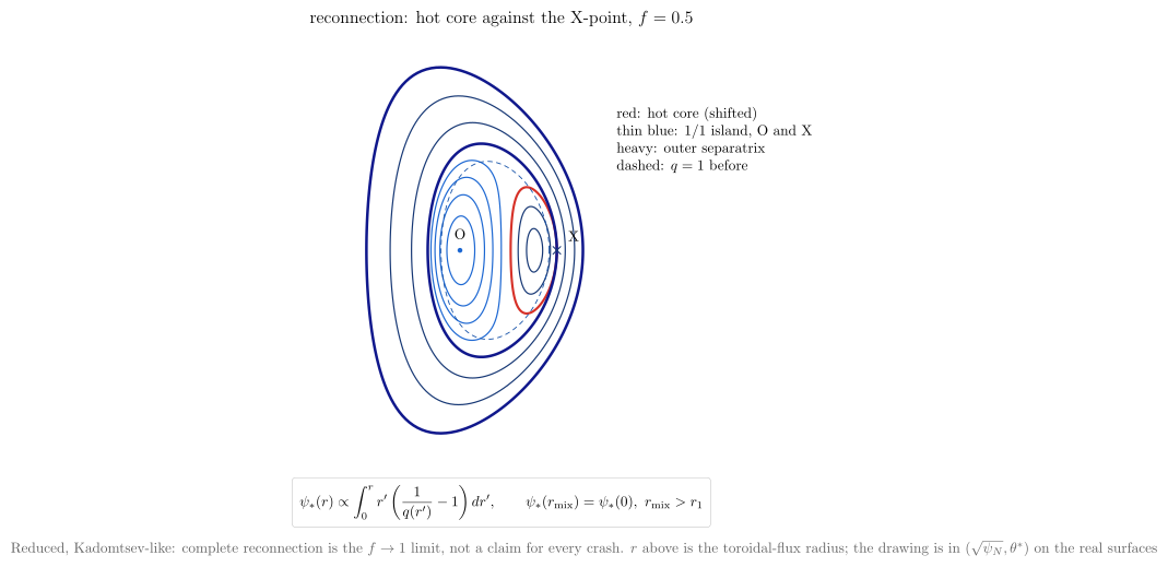
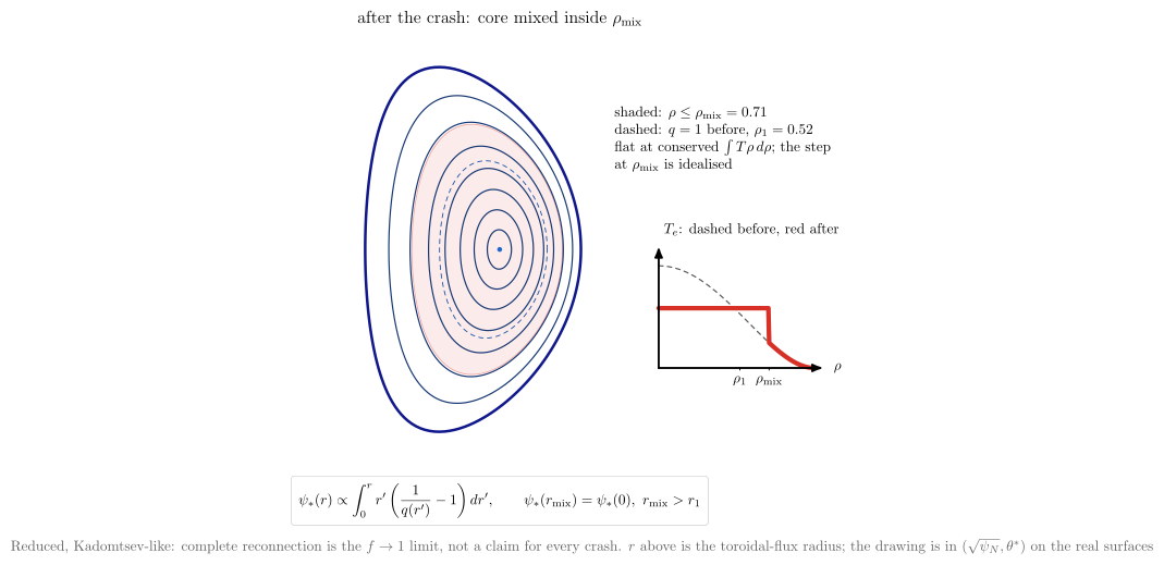
vaft.diagram.sawtooth(stage="precursor")   # "reconnection", "post_crash"
 |
 |
 |
 |
| Diagram | Model class | Concept |
|---|---|---|
kink_mode |
synthetic parameterization | Each surface moves along its normal by $\xi_n = A\,a\,F(\rho)\,\mathrm{Re}\sum c_m e^{i(m\theta^* - n\phi)}$, with a named envelope. internal is a top hat inside $q = m/n$, global is $\rho^{m-1}$, and edge is $\rho^{4m}$. Under flux freezing this is flux_perturbation_from_normal_displacement, $\delta\psi = -\xi_n\lvert\nabla\psi\rvert$. It is not an eigenfunction. The cylindrical reference view is internal_external_kink |
sawtooth |
reduced model | precursor: the 1/1 internal kink inside $q = 1$, with nested topology kept. reconnection: a hot core of radius $\rho_1(1-f)$ pushed against an outer separatrix, with the X-point where they touch and the 1/1 island in the crescent between. post_crash: nested surfaces again, with the region inside the Kadomtsev mixing radius flattened at conserved $\int T\rho\,d\rho$ |
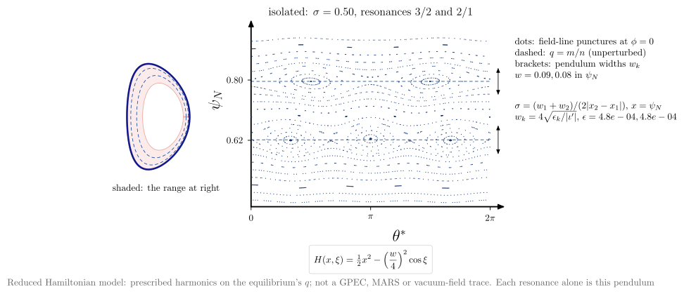
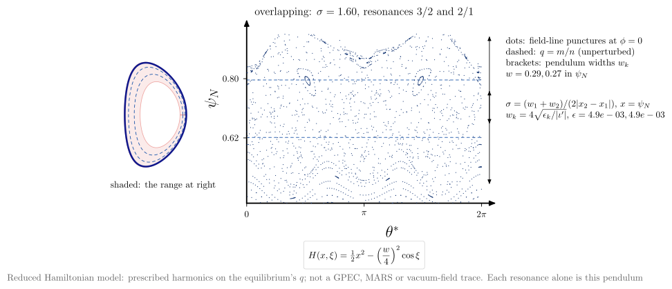
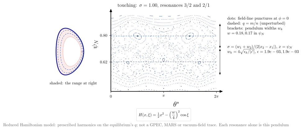
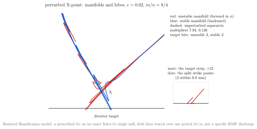
Two reduced Hamiltonian models extend the vocabulary of magnetic_island to several resonances, and to the
X-point.
vaft.diagram.stochastic_layer(regime="touching")   # "isolated", "overlapping"; or overlap=, perturbations=
vaft.diagram.separatrix_lobes(perturbation=0.02, m=8, n=4)       # or separatrix_lobes(equilibrium, ...)
 |
 |
| Diagram | Model class | Concept |
|---|---|---|
stochastic_layer |
reduced Hamiltonian | A Poincaré section of $H = \int\iota\,d\psi_N - \sum_k\epsilon_k\cos(m_k\theta^* - n_k\phi)$ on the equilibrium’s $q$ (default 3/2 and 2/1). Each resonance alone is the pendulum of island_pendulum_hamiltonian, width $4\sqrt{\epsilon/\lvert\iota’\rvert}$. The pair overlap $\sigma$ (vaft.process.perturbation.chirikov) is 0.5, 1 or 1.6. The inset shows where the section sits |
separatrix_lobes |
reduced Hamiltonian | A lower-single-null equilibrium (by default the single-null Solov’ev) plus a prescribed $\delta\psi \propto (r/r_X)^m\cos(m\vartheta - n\phi)$. The field-line map over $2\pi/n$ has a hyperbolic fixed point (Newton, multipliers $\lambda$ and $1/\lambda$). Its unstable and stable manifolds split from the unperturbed separatrix and cross each other, which makes lobes, and one strike point on the target becomes several |
In stochastic_layer, $x = \psi_N$ stands in for the toroidal-flux action, so $\epsilon$ is a model amplitude and area in the section is not flux. separatrix_lobes takes any lower-single-null EquilibriumData: the X-point must be a saddle of the flux on the boundary value, below the axis, and the window scales with the minor radius; a limited equilibrium is refused. Neither diagram is a GPEC, MARS or vacuum-field trace: those belong to result plotting.
The mixing radius comes from vaft.formula.kadomtsev_mixing_radius: the 1/1 helical flux
$\psi_* \propto \int r(1/q - 1)\,dr$ returns to its axis value there. It equals $\sqrt2\,r_1$ when
$1/q - 1$ is parabolic. Complete (Kadomtsev) reconnection is the $f \to 1$ limit, not a claim about every
crash.
MARFE
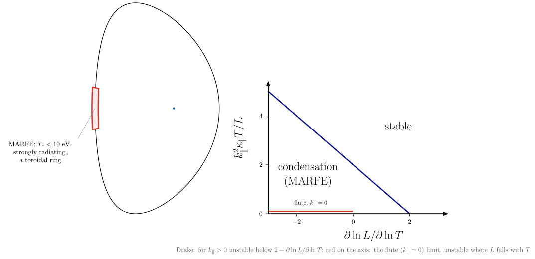
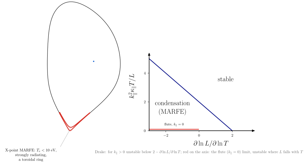
marfe puts a prescribed radiation condensation on the edge of an equilibrium and shows the condition that
makes it.
- On the high-field side (
localization="hfs", the usual location) the band straddles the last closed surface. It is about 30° wide poloidally and 0.1$a$ deep, as Lipschultz (1987) reports. - Next to the X-point (
"xpoint", Greenwald 2002 p. R35) the band is drawn on the closed side with the same sizes, which are borrowed, not measured there. - Its $T_e$ is below about 10 eV (Greenwald p. R34), and it is toroidally symmetric: a ring.
The right panel is Drake’s (1987) constant-pressure criterion in dimensionless form, computed from
vaft.formula.sol.radiative_condensation_growth_rate. For $k_\parallel > 0$ the boundary is
$k_\parallel^2\kappa_\parallel T/L = 2 - \partial\ln L/\partial\ln T$, so condensation does not need a
falling radiation curve. On the $k_\parallel = 0$ axis only the constant-density flute limit
(radiative_thermal_instability_growth_rate) applies, and it is unstable where $L$ falls with $T$.
The band is prescribed, not solved, and no cooling curve or density-limit formula is built in; MARFE onset
and density-limit semantics belong to #1068. The API names its sizes poloidal_width_deg and
radial_fraction; the issue’s "prescribed" localization is not implemented.
vaft.diagram.marfe(localization="hfs") # or "xpoint"; poloidal_width_deg=30, radial_fraction=0.1
 |
 |
Divertor heat-flux footprint
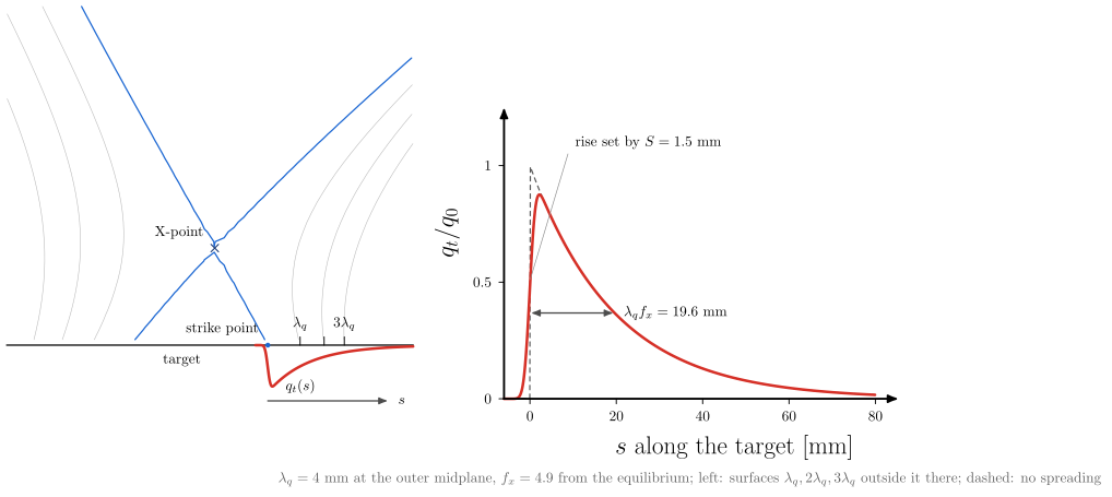
divertor_heat_footprint maps an Eich target profile onto a diverted equilibrium. The geometry comes from
the equilibrium itself: the X-point is the zero of $\nabla\psi$ next to the lowest boundary point, the
strike point is where the separatrix leg crosses a horizontal target, and the total flux expansion
$f_x = (\partial\psi/\partial R)\mathrm{OMP} / (\partial\psi/\partial s)\mathrm{target}$ is
evaluated on the flux, not assumed. The profile is vaft.formula.sol.eich_target_heat_flux_profile with
that $f_x$. $\lambda_q$ (at the outer midplane) and $S$ (at the target) are illustrative inputs: this is a
schematic, and measured IR profiles belong in vaft.plot. The SOL surfaces one, two and three $\lambda_q$
outside the separatrix at the midplane fan out to about $k\lambda_q f_x$ on the target. The equilibrium must be
lower single null, with an X-point on its boundary flux and legs that reach the target inside the limiter;
anything else is refused rather than drawn.
vaft.diagram.divertor_heat_footprint(lambda_q=0.004, spreading=0.0015, target="outer")
Disruption physics: quench sequence, runaways and energy paths
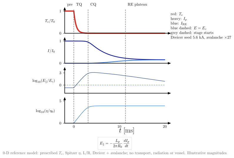
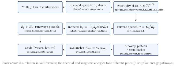
The chain from loss of confinement to a runaway plateau, each link a relation in the new
vaft.formula.disruption category or an existing one:
thermal_quench_temperature,current_quench_currentandinductive_parallel_electric_field;connor_hastie_critical_field,dreicer_field,runaway_critical_momentumandrelativistic_collision_time;dreicer_generation_rate,avalanche_growth_rate,avalanche_efolds_from_current_dropandrunaway_current_from_density;- the Spitzer resistivity, and the
startupplasma resistance, inductance and L/R time.
Detecting a disruption in data stays in vaft.process.transients. Simulating one belongs to kinetic or
integrated codes.
vaft.diagram.disruption_timeline()
vaft.diagram.disruption_causal_chain()
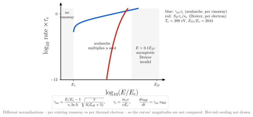
vaft.diagram.runaway_generation()
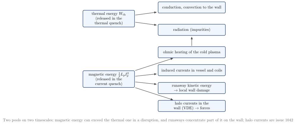
vaft.diagram.disruption_energy_pathways()
 |
 |
| Diagram | Concept |
|---|---|
disruption_timeline |
A 0-D reference model built from the formulas. A prescribed thermal quench raises the Spitzer $\eta$. The L/R current quench then induces $E_\parallel \approx 10^3E_c$ ($\approx 2\,\%$ of $E_D$). A Dreicer seed of a few kA is multiplied about 25-fold by the avalanche (at 1 MA, only a few e-folds) into a runaway plateau. Magnitudes are illustrative: no universal waveform |
disruption_causal_chain |
The same sequence as cause and effect, each arrow labelled by its formula |
runaway_generation |
The avalanche rate (per runaway) and the Dreicer rate (per electron) against $E/E_c$. The normalisations differ, so the two magnitudes are not compared. Nothing runs away below $E_c$, and Dreicer is drawn only within its asymptotic range, $E \le 0.1E_D$. Hot-tail seeding is not drawn |
disruption_energy_pathways |
Thermal energy leaves by conduction and radiation. Magnetic energy $\tfrac12L_pI_p^2$ goes to ohmic heating, the vessel and coils, runaway kinetic energy and halo currents (#1042). The existing thermal_energy_from_p_V, virial_thermal_energy and magnetic_energy_from_li_B_pa_V_p compute the two pools |
Vertical displacement events: hot and cold VDE, halo currents
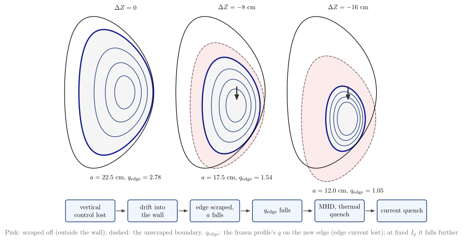
A hot VDE moves a still-hot plasma into the wall, and the scraping can trigger the thermal quench. A cold
VDE follows the quench, as the decaying current loses its centred vertical equilibrium. Wall contact then
drives halo currents through the scrape-off layer and the wall. The model-neutral reference quantities are
in the new vaft.formula.vde category:
vertical_velocityandvde_growth_rate(a local $d\ln\lvert\Delta Z\rvert/dt$);thin_wall_timeandwall_mode_decay_time;halo_current_fractionandtoroidal_peaking_factor.
A wall element’s $L/R$ is lr_time_from_L_R. The named reduced VDE models (edge-current loss,
filament-plus-wall, analytic halo) are not chosen yet. The disruption chain these diagrams couple to is
vaft.formula.disruption.
vaft.diagram.hot_vde_sequence()
vaft.diagram.cold_vde_bifurcation()
vaft.diagram.plasma_wall_halo_current()
vaft.diagram.vde_timescales()
 |
 |
| Diagram | Concept |
|---|---|
hot_vde_sequence |
The Solov’ev plasma moved 0, 8 and 16 cm into its limiter. The limiting surface shrinks, so the edge moves inward to lower $q$ (the equilibrium’s own profile; the cylindrical estimate at fixed $I_p$ falls as $a^2$). Below, the causal chain towards the thermal quench |
cold_vde_bifurcation |
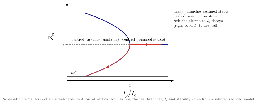
A schematic normal form: below a critical current the centred equilibrium is lost, and the plasma follows an off-centre branch into the wall as $I_p$ decays. The real branches come from a model not chosen here |
plasma_wall_halo_current |
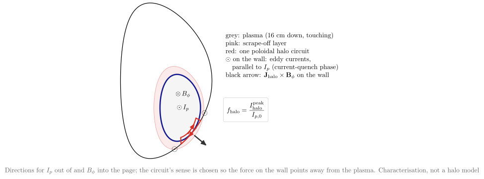
Poloidal halo current through the scrape-off layer and the wall, toroidal eddy currents in the wall, and $\mathbf J_\mathrm{halo}\times\mathbf B_\phi$ on the floor, for one sign of $I_p$ and $B_\phi$ |
vde_timescales |
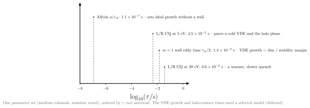
$a/v_A$, the $m = 1$ wall time, and the L/R current-quench time at 5 and 20 eV for one medium-tokamak parameter set. The ordering is not universal |
Plasma-wall interaction
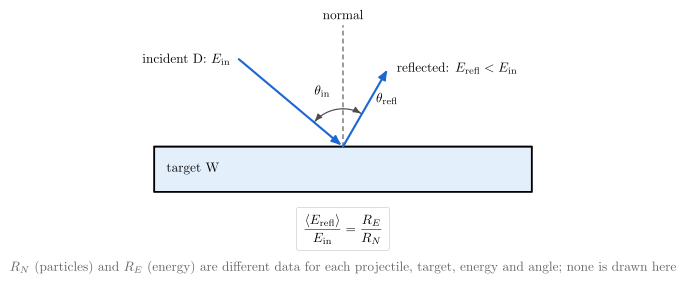
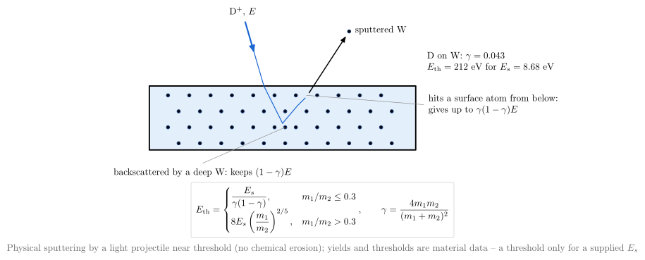
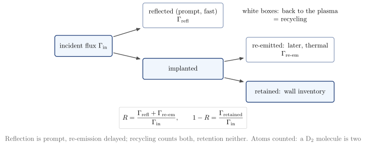
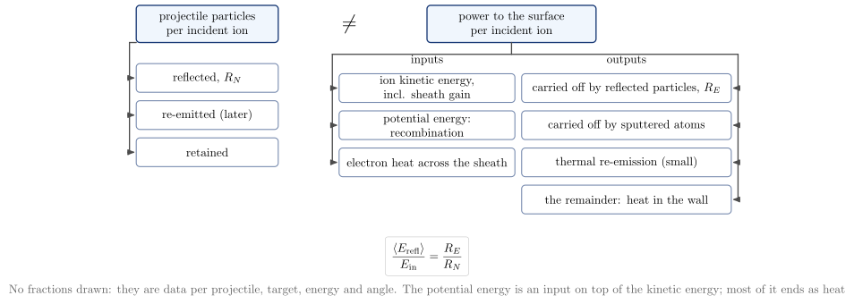
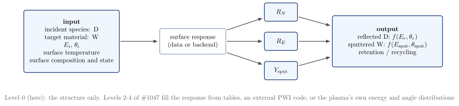
The plasma-wall vocabulary: one impact and its outcomes, reflection (particle versus energy), physical
sputtering, recycling versus retention, and particle versus energy balance. This is level 0 of the
issue’s enrichment, semantics only. No reflection or sputtering coefficient, yield or threshold is drawn
unless it is computed by a vaft.formula.pwi relation from inputs the caller supplies:
binary_collision_energy_transfer_factor, the exact elastic kinematics;mean_reflected_energy_fraction, which is $R_E/R_N$;recycling_coefficient;sputtering_threshold_bohdansky, a named empirical fit that needs the surface binding energy.
Projectile and target species go through vaft.data.atomic and are drawn apart: projectile blue,
target dark. Each diagram’s model names the IMAS paths of the quantities it shows, under
wall.global_quantities.neutral[:]: the recycling particle and energy coefficients, the fluxes from the
plasma and from the wall, the wall inventory, and the per-incident-species sputtering coefficients.
IMAS’s recycling energy coefficient covers all recycling channels, so it is not the prompt-reflection
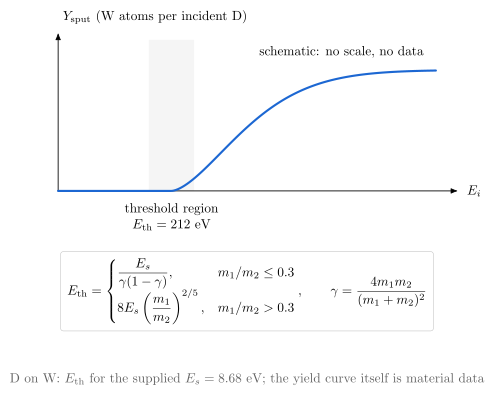
$R_E$. The canonical sputtering figure uses $E_s = 8.68$ eV, the sublimation energy of W, as a stated input.
vaft.diagram.plasma_wall_interaction_processes(projectile="D", target="W")
vaft.diagram.plasma_wall_interaction_reflection()
vaft.diagram.plasma_wall_interaction_sputtering(surface_binding_energy=8.68)   # threshold only if E_s given
vaft.diagram.plasma_wall_interaction_recycling()
vaft.diagram.plasma_wall_interaction_energy_partition()
vaft.diagram.plasma_wall_interaction_reflection_energy()
vaft.diagram.plasma_wall_interaction_angle_dependence()
vaft.diagram.plasma_wall_interaction_sputtering_threshold(surface_binding_energy=8.68)   # E_th only if E_s given
vaft.diagram.plasma_wall_interaction_particle_balance()
vaft.diagram.plasma_wall_interaction_surface_response()
 |
 |
 |
 |
 |
 |
 |
 |
| Diagram | Concept |
|---|---|
plasma_wall_interaction_processes |
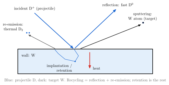
Reflection (fast atom), implantation and retention, re-emission (thermal molecule), sputtering (target atom), and heat |
plasma_wall_interaction_reflection |
$E_\mathrm{in}$, $E_\mathrm{refl}$, $\theta_\mathrm{in}$ and $\theta_\mathrm{refl}$ as separate quantities; $R_N$ is not $R_E$ |
plasma_wall_interaction_sputtering |
A collision cascade ejects a target atom. One collision passes at most $\gamma E$ (D on W: $\gamma = 0.043$), hence the high threshold |
plasma_wall_interaction_recycling |
Prompt reflection plus delayed re-emission make recycling; retention is the rest |
plasma_wall_interaction_energy_partition |
Particle balance and energy balance side by side. They are not the same bookkeeping |
plasma_wall_interaction_reflection_energy |
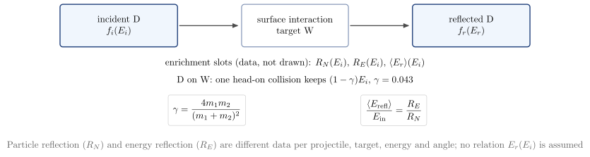
Incident $f_i(E_i)$ to reflected $f_r(E_r)$ through the surface. Only the binary-collision limit $(1-\gamma)E_i$ is stated; $R_N(E_i)$, $R_E(E_i)$, $\langle E_r\rangle(E_i)$ are empty enrichment slots |
plasma_wall_interaction_angle_dependence |
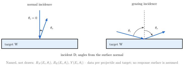
Normal and grazing incidence, angles from the surface normal; $R_N$, $R_E$, $Y$ as functions of $(E_i, \theta_i)$ are named, not drawn |
plasma_wall_interaction_sputtering_threshold |
A schematic $Y(E_i)$ with no scale: a threshold exists. $E_\mathrm{th}$ is printed only for a supplied $E_s$ (Bohdansky) |
plasma_wall_interaction_particle_balance |
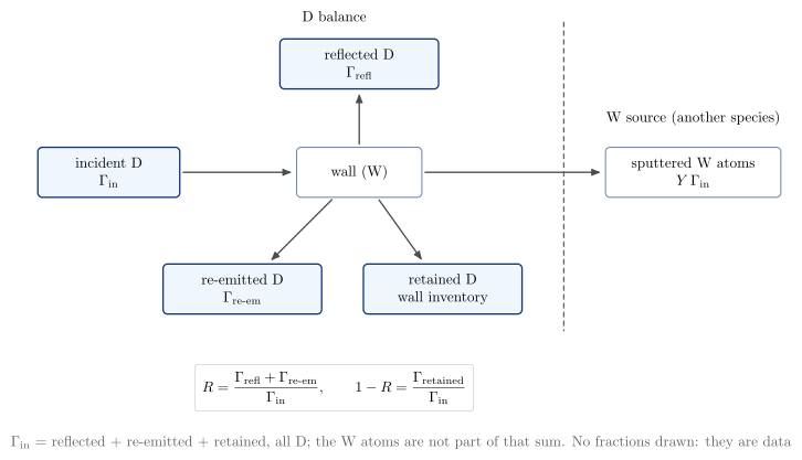
The projectile balance (reflected + re-emitted + retained) with the sputtered target atoms drawn apart, as another species’ source |
plasma_wall_interaction_surface_response |
Inputs, surface response ($R_N$, $R_E$, $Y_\mathrm{sput}$), outputs: the extension point for tabulated data or an external PWI code (levels 2–4) |
Spectroscopy and ionization
Concept diagrams in the vocabulary of vaft.data.atomic and vaft.data.spectroscopy. parse_emission_term and parse_line_label are
the same parsers emission= uses in vaft.plot, so a term that selects a trace selects the same diagram.
Metadata is progressive, and nothing is fabricated:
- level 0 is the semantic identity (stage, charge, element);
- level 1 is what the data declare (the wavelength in an IMAS
processed_linelabel such asOI_7770); - hydrogenic lines add Bohr-model levels and Rydberg vacuum wavelengths with the isotope’s reduced mass
(
hydrogenic_energy_levelandhydrogenic_transition_wavelengthinvaft.formula.atomic). For one-electron systems this model is the authoritative source; each model records it undersource; - many-electron levels and photon emissivities would need OPEN-ADAS ADF04 and ADF15. Those are extension
points and are not loaded; ADF11 stays in
vaft.formula.atomic.
vaft.diagram.spectroscopy_ionization_stages("C III")   # "C2+", "carbon", "CIII_1909" too
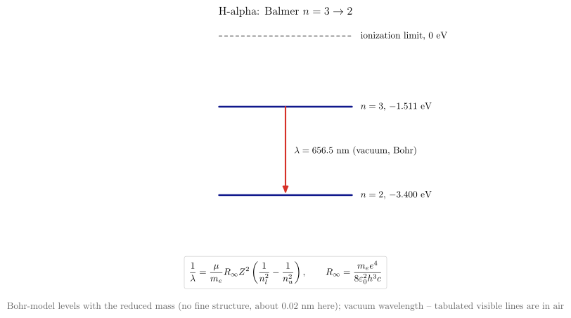
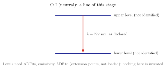
vaft.diagram.spectroscopy_transitions("H-alpha")        # "OI_7770": declared wavelength only
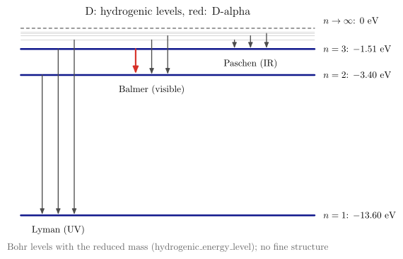
vaft.diagram.spectroscopy_energy_levels("D-alpha")
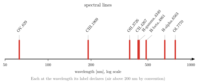
vaft.diagram.spectroscopy_spectrum()                    # the labels VEST's spectrometer declares

 |
 |
| Diagram | Concept |
|---|---|
spectroscopy_ionization_stages |
Every stage of an element, with the named one outlined. Stage $s$ is charge $s - 1$, and D and T are hydrogen with a mass number. Semantic only |
spectroscopy_transitions |
A hydrogen series member gets Bohr-model levels and its vacuum wavelength (an unspecified isotope is taken as protium, and the title says so). Fully stripped ions are refused, since they have no lines. Any other line gets unnamed levels, and a wavelength only if its label declares one |
spectroscopy_energy_levels |
The hydrogenic ladder with the Lyman, Balmer and Paschen series. Hydrogenic only: other species need ADF04 |
spectroscopy_spectrum |
Declared lines, each at its label’s wavelength (air above 200 nm by convention). Computed hydrogenic lines are dashed and in vacuum. Lines with no wavelength are listed, not placed |
Neutral beam injection: lifecycle and reduced attenuation
A small, machine-independent NBI layer. It is not NUBEAM, ASCOT5 or BEAMS3D, and it never replaces
vaft.code.nubeam.
- Formulas (
vaft.formula.nbi):beam_particle_rate_from_power_energy(per energy component, in eV),neutral_beam_optical_depth,neutral_survival_fraction_from_optical_depth,beam_birth_probability_density(a density along the path, not a volumetric deposition),shine_through_fraction, andinjected_toroidal_angular_momentum_rate. The last is the ideal rate carried in, not the torque on the plasma. - Process (
vaft.process.nbi.neutral_beam_attenuation_along_path): composes these along a prescribed 1-D path and adds the particle and power bookkeeping. Births are counted per path cell as $S_i - S_{i+1}$, so $\sum_i + f_\mathrm{shine} = 1$ and $P_\mathrm{birth} + P_\mathrm{shine} = P_\mathrm{injected}$ hold exactly on any grid. The “power birth profile” is where neutrals become fast ions, not where the plasma is heated. The process module’s docstring tabulates what this layer answers and what needs a full solver; related work is #265 (VEST NBI description), #592 (NUBEAM → IMAS), #1064 and #1092 (scales, orbits).
The attenuation coefficient $\alpha = \sum_j n_j\sigma_j$ is always an input; no beam-stopping data are built in. Orbits, trapped and passing fast ions, and $P_\phi$ are the particle-motion diagrams’, and are not redrawn here.
vaft.diagram.nbi_particle_lifecycle()      # shine-through / prompt loss / delayed loss kept apart
vaft.diagram.nbi_neutral_attenuation()     # S(s), b(s), births and f_shine from vaft.formula.nbi
Iteration behaviour, branch bifurcation and branch selection
Non-convergence can arise from true branch structure or from numerical cycling. A solver that does not converge has not necessarily found an unphysical solution, and these diagrams separate the cases. They are generic concept diagrams for EFIT convergence, grid, weighting and continuation studies. No shot, residual or grid comparison is shown or implied, and none of them claims that a physical bifurcation exists in VEST equilibria.
Every curve is computed:
- the iteration panels come from the logistic map $x_{k+1} = rx_k(1 - x_k)$ at $r = 2.8$, $3.2$ and $3.5$, and from an expanding linear map;
- the branch diagram is the saddle-node normal form $\dot x = \lambda + x - x^3$;
- the basins are its exact relaxation at $\lambda = 0$.
The bifurcation is drawn once. The basin diagram is the same model at one control parameter, not a second bifurcation figure.
vaft.diagram.iteration_behavior()       # fixed point, divergence, 2-cycle, period-4 limit cycle
vaft.diagram.branch_bifurcation()       # stable (solid) / unstable (dashed), folds, jumps, hysteresis
vaft.diagram.basin_of_attraction()      # initial condition selects branch A or B
vaft.diagram.grid_induced_two_cycle()   # each re-solve lands nearer the other node: a one-cell hop
vaft.diagram.branch_selection()         # the last two side by side under one caption
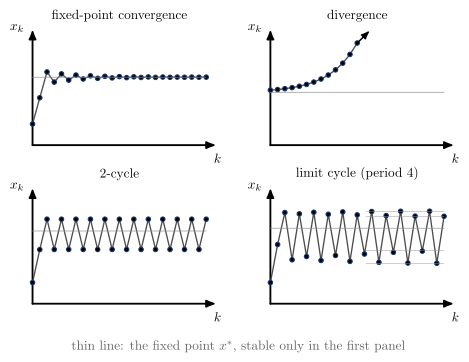
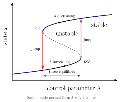 |
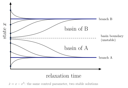 |
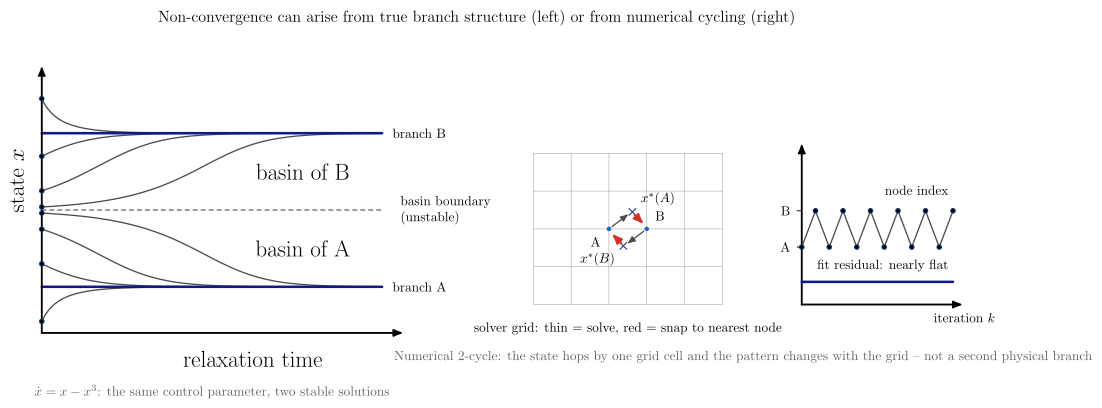
| Diagram | Concept |
|---|---|
iteration_behavior |
$x_k$ against $k$ in one format. The fixed point $x^*$ (thin line) exists in every panel but is stable only in the first; guides mark the four levels of the period-4 cycle |
branch_bifurcation |
Stable and unstable branches, the two folds, the jump at each fold, and the hysteresis loop; three equilibria coexist between the folds |
basin_of_attraction |
Two stable solutions at one control parameter. The unstable equilibrium is the basin boundary, and the start decides the branch |
grid_induced_two_cycle |
A numerical artifact. Solved from A the optimum lands nearer B, and from B nearer A, so the index hops by one grid cell and the pattern changes with the grid. The fit stays nearly flat (a secondary cue). It is not a second physical branch |
branch_selection |
basin_of_attraction beside grid_induced_two_cycle: physical branch structure against numerical cycling |
Cold-plasma waves: dispersion, cutoffs, resonances and the CMA diagram
Each diagram is drawn from the cold-plasma equations in vaft.formula.waves:
plasma_frequency;stix_parameters, giving $R, L, S, D, P$ with the signed cyclotron frequency, so $\Omega_e < 0$, anddielectric_tensor;cold_plasma_refractive_index_squared, the two roots of $An^4 - Bn^2 + C = 0$, in a cancellation-free form that keeps the finite root at a resonance cone;perpendicular_refractive_index_squared, giving $n_O^2 = P$ and $n_X^2 = RL/S$;-
cma_coordinates, giving $X = \omega_{pe}^2/\omega^2$ and $Y =\Omega_e /\omega$; propagation_regime, which classifies propagating, evanescent, cutoff and resonance.
Boundaries are zeros or poles of the Stix parameters, located by bracketing the formulas; no closed form is typed into a drawing. The $\pm$ roots are algebraic branches, not mode names, so O/X and R/L are named only where the mode is tracked: at $\theta = \pi/2$ and $\theta = 0$. Electrons only, ions immobile: the electron-cyclotron range. Warm-plasma effects, damping, ray tracing and full-wave solutions are out of scope.
import math

vaft.diagram.o_mode_cutoff()                                  # n_O^2 = P, cutoff at omega_pe
vaft.diagram.x_mode_dispersion(omega_pe_over_omega_ce=1.2)    # L, R cutoffs; upper-hybrid resonance
vaft.diagram.cma_diagram()                                    # P, R, L, S = 0 and Y = 1 in (X, Y)
vaft.diagram.profile_propagation()                            # layers along an example midplane
vaft.diagram.profile_propagation(theta=math.radians(60))      # oblique: both roots, A = 0 resonances
vaft.diagram.wave_dispersion_omega_k(omega_pe_over_omega_ce=1.2)  # branches in the omega-k plane
vaft.diagram.refractive_index_vs_X(Y=0.5)                     # rising density at fixed field
vaft.diagram.refractive_index_vs_Y(X=0.5)                     # rising field at fixed density
Every view takes theta, from $5^\circ$ to $\pi/2$ (below that, parallel propagation is the picture). At $\theta = \pi/2$ the branches are named O (blue) and X (red). At any other
angle both roots of cold_plasma_refractive_index_squared are drawn in one colour, because the algebraic
$\pm$ branches swap at the cyclotron layer, and the resonance moves from $S = 0$ to the cone
$A = S\sin^2\theta + P\cos^2\theta = 0$, which is marked.
Neoclassical and NTV collisionality regimes
Two different regime families that share the word “collisionality”. Axisymmetric neoclassical transport orders the collision frequency against the transit and bounce frequencies. Neoclassical toroidal viscosity (NTV) in broken symmetry orders it against the bounce-averaged precession $\omega_d = \omega_E + \omega_B$:
Coulomb collisions -> transit / bounce motion -> nu_hat = qR nu/v -> banana / plateau / Pfirsch-Schlueter
3-D delta B + precession omega_d -> 1/nu / nu-sqrt(nu) / superbanana-plateau / nu -> NTV torque
The axis of the first diagram is $\hat\nu = qR_0\nu/v$ (collisions_per_transit), not a $\nu_$. VAFT’s
several $\nu_$ conventions (issue 353) share the symbol but not the value. The boundaries
$\hat\nu = \epsilon^{3/2}$ and $1$ come from neoclassical_regime_boundaries. The orbit scales behind
them are transit_frequency, deeply_trapped_bounce_frequency,
trapped_particle_effective_collision_frequency and banana_width in vaft.formula.neoclassical.
vaft.formula.ntv holds the exact, convention-bearing relations:
ntv_precession_frequency, whose zero is the superbanana-plateau resonance. $\omega_E$ is the $E\times B$ frequencyomega_exb, never the toroidal rotation, and both $\omega_E$ and $\omega_B$ are measured along the plasma current;nonambipolar_torque_density, the torque on the plasma: the $\mathbf J\times\mathbf B$ of the return current that cancels the non-ambipolar flux. Ion loss in a co-current plasma drives counter-current rotation.
The size of the flux needs a drift-kinetic code (vaft.code), and Shaing’s connected formula is not
implemented, so the NTV regime diagram shows slopes only.
vaft.diagram.neoclassical_collisionality(epsilon=0.1)
vaft.diagram.ntv_collisionality()
vaft.diagram.ntv_precession_regimes(omega_magnetic=1.0)
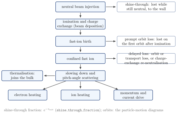 |
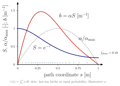 |
| Diagram | Concept |
|---|---|
nbi_particle_lifecycle |
Injection, ionisation, fast-ion birth, confinement, slowing down, heating and drive, then thermalisation. Each loss branches at its own stage: shine-through while neutral, prompt orbit loss after ionisation, delayed loss after confinement |
nbi_neutral_attenuation |
Survival $e^{-\tau}$ and birth density $\alpha S$ along a path through a parabolic plasma (an illustrative $\alpha$). Births are drawn at equal probability steps, and the shine-through is marked at the exit |
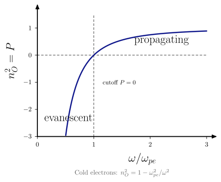 |
 |
 |
 |
 |
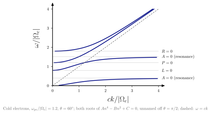 |
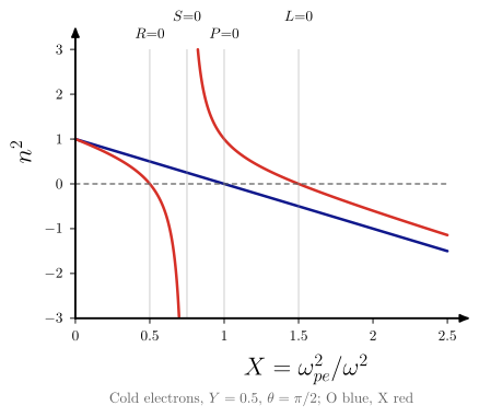 |
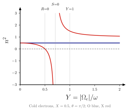 |
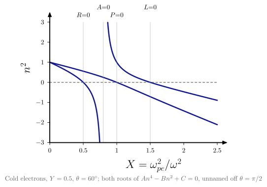 |
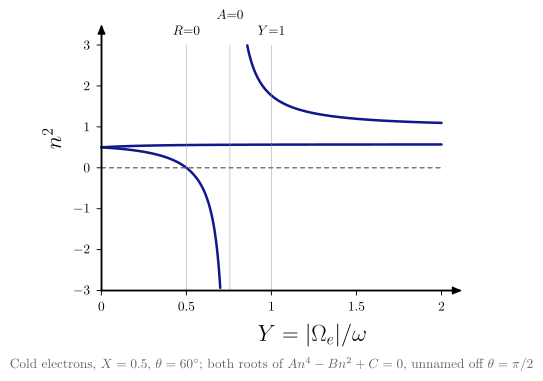 |
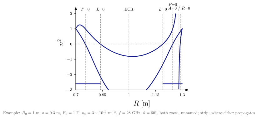 |
| Diagram | Concept |
|---|---|
o_mode_cutoff |
Evanescent below $\omega_{pe}$, propagating above; the cutoff $P = 0$ does not depend on $B$ |
x_mode_dispersion |
Evanescent below $\omega_L$, propagating to the upper-hybrid pole, evanescent to $\omega_R$, then propagating. Poles are masked |
cma_diagram |
Cutoffs (solid) and resonances (dashed) of a cold electron plasma in the CMA plane |
profile_propagation |
$n_O^2$ and $n_X^2$ along $R$, with strips where each mode propagates (propagation_regime), for an example tokamak (not a device) at the on-axis electron cyclotron frequency: O cutoffs, L and R cutoffs, the upper-hybrid layer behind the R cutoff, and the ECR. With theta, both oblique roots and the $A = 0$ layers |
wave_dispersion_omega_k |
Each branch in the $\omega$-$k$ plane ($k = n\omega/c$ where $n^2 > 0$): it starts at $k = 0$ on its cutoff ($P$, $R$ or $L = 0$) – the oblique whistler leaves the origin instead – runs to $k \to \infty$ at a resonance, and approaches the light line at high frequency |
refractive_index_vs_X |
$n^2$ against $X$ at fixed $Y$: cutoffs at $X = 1 - Y$ ($R$), $1$ ($P$), $1 + Y$ ($L$), the upper hybrid at $X = 1 - Y^2$, all located by bracketing |
refractive_index_vs_Y |
$n^2$ against $Y$ at fixed $X$: at $\theta = \pi/2$ the O branch does not depend on $Y$; the other has the $R$ cutoff at $Y = 1 - X$, the upper hybrid at $\sqrt{1 - X}$, and $Y = 1$ is the cyclotron layer |
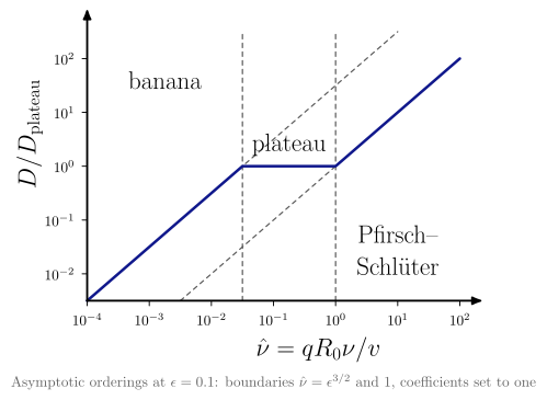 |
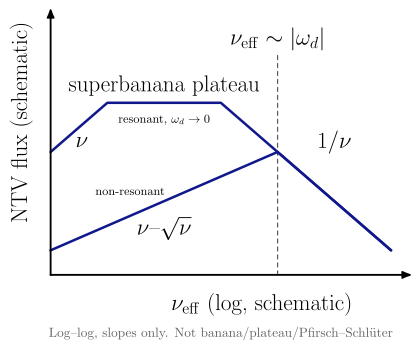 |
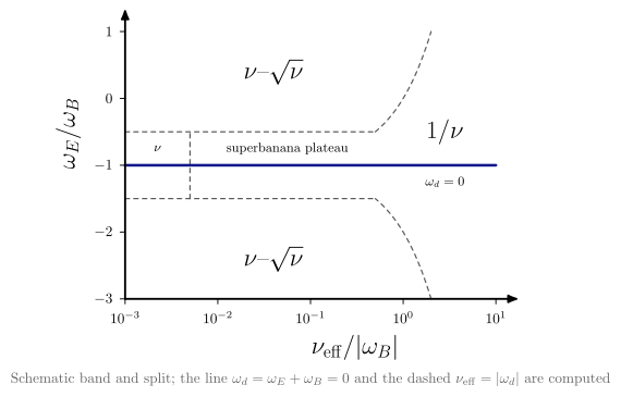 |
| Diagram | Concept | ||
|---|---|---|---|
neoclassical_collisionality |
$D/D_\mathrm{plateau}$ against $\hat\nu$: asymptotes $\hat\nu/\epsilon^{3/2}$, 1 and $\hat\nu$ meeting at the formula’s boundaries. Orderings, not phase boundaries | ||
ntv_collisionality |
Non-resonant ($1/\nu$, then $\nu$–$\sqrt\nu$) and resonant ($1/\nu$, superbanana plateau, superbanana $\nu$) branches, with Shaing’s exponents. Schematic breakpoints | ||
ntv_precession_regimes |
$\nu_\mathrm{eff}$ against $\omega_E/\omega_B$: the resonance $\omega_d = 0$ and the ordering $\nu_\mathrm{eff} = | \omega_d | $ from ntv_precession_frequency. A schematic resonant band holds the superbanana plateau and $\nu$ regimes |
Wall conditioning
Baking, glow-discharge cleaning and boronization, each drawn as a transition of the wall state
$S^{(0)}\mathrm{wall} \to S^{(1)}\mathrm{wall}$ (WALL_STATE_CHANGE in the module), not only as
“cleaning”. The diagrams are reduced and semantic, and share one vessel with an inlet port, a pump port
and a wall-surface primitive:
- baking is thermal desorption only: no glow, anode, ion bombardment or coating;
- the glow discharges share one apparatus template: gas feed, glow, anode, the wall as cathode, and ions accelerated across the cathode sheath onto the whole wall. H$_2$/D$_2$ is reactive cleaning, with volatile O/C products that match the feed isotope. He is ion-induced release of retained H/D, drawn with its own arrow style;
- boronization names a “B-containing precursor” unless one is passed, and leaves a B-rich layer.
Species are examples. No temperature, precursor, pressure or thickness is built in. A temperature (in K or °C) or a thickness is drawn only when the caller passes it together with its source. The sequence ends in plasma operation; how the conditioned wall responds then is the plasma-wall interaction section.
vaft.diagram.wall_conditioning_baking()        # temperature=, temperature_unit="K"|"degC", temperature_source=
vaft.diagram.wall_conditioning_gdc("D2")       # "H2", "D2" or "He"
vaft.diagram.wall_conditioning_boronization(precursor="B$_2$H$_6$")
vaft.diagram.wall_conditioning_sequence(("baking", "D2_gdc", "He_gdc", "boronization"))

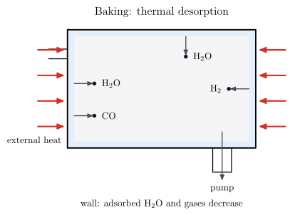 |
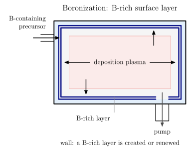 |
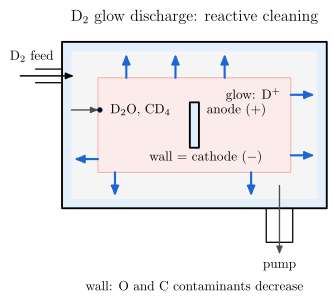 |
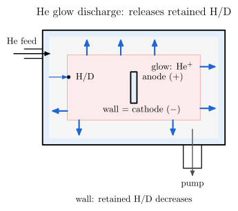 |
| Diagram | Concept |
|---|---|
wall_conditioning_baking |
External heat drives adsorbed water and gases off the wall into the pump |
wall_conditioning_gdc |
One glow-discharge template. H$_2$/D$_2$: O and C leave as volatile products. He: He$^+$ bombardment releases retained H/D |
wall_conditioning_boronization |
A B-containing precursor in a deposition plasma leaves a B-rich surface layer, a change of surface state rather than cleaning |
wall_conditioning_sequence |
The single stages in the caller’s order, each arrow a wall-state transition, ending in plasma operation. The order is not a recommended procedure |
SOL blobs and filaments
A blob is a localized positive density (pressure) perturbation in the scrape-off layer, and a hole is a negative one. The filament is the field-aligned structure whose perpendicular cross-section is the blob.
How a blob moves:
- curvature and $\nabla B$ drift ions and electrons apart;
- the density monopole becomes a charge dipole, $+$ above and $-$ below;
- the dipole’s $E$ field drives an $E\times B$ drift outward on the low-field side, down $\nabla B$ (a hole moves inward).
How fast it moves depends on where the polarization current closes:
- along the field to the sheaths (sheath-connected, $v \propto \delta^{-2}$);
- across the field by ion inertia (inertial or resistive-ballooning, $v \propto \delta^{1/2}$);
- with resistivity and X-point fanning, in between.
vaft.formula.sol holds the prescribed filament state blob_density_perturbation (a blob, or a hole below
the background), the reference size $\delta_* = \rho_s^{4/5}L_\parallel^{2/5}/R^{1/5}$, the
reference velocity $v_$, the collisionality $\Lambda$, both limits, the interpolation, and the four regime
scalings. All follow D’Ippolito, Myra and Zweben (2011), with a Gaussian of radius $\delta$. The $O(1)$
prefactors in Krasheninnikov (2001) and Theiler et al. (2011) belong to their own size definitions. The NSTX
parameters of Myra et al. (2006) give $\hat a \approx 1.3$, as in their Fig. 1, and $v_ \approx 3$ km/s from their
symbolic Eq. (3); their text quotes $v_* \sim 2$ km/s. Cold ions throughout: $c_s = (T_e/m_i)^{1/2}$.
vaft.diagram.blob_polarization()        # the mechanism: dipole, E, E x B; perturbation="hole" reverses it
vaft.diagram.blob_current_closure(regime="sheath")   # or "inertial": where the current closes
vaft.diagram.blob_velocity_scaling()    # v/v* against delta/delta*: both limits and Eq. (9)
vaft.diagram.blob_regimes(epsilon_x=0.1)  # Lambda against Theta = delta_hat^{5/2}: RB, RX, C_i, C_s
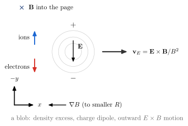 |
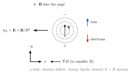 |
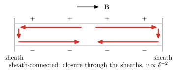 |
 |
 |
 |
The VAFT framework: pillars, research cycle, managed pipeline, provenance
These diagrams describe what VAFT is and how scientific data moves through it (#1090). They work at the level of scientific capabilities, not deployment: no storage backend, endpoint, path or module name appears in them, and a test enforces this. The README uses the four pillars, the research cycle and the managed pipeline.
vaft.diagram.vaft_four_pillars()
vaft.diagram.fusion_science_knowledge_lifecycle()
vaft.diagram.scientific_workflow()
vaft.diagram.interoperability_layers()
vaft.diagram.scientific_provenance_chain()
vaft.diagram.plasma_state_provenance()
vaft.diagram.scientific_infrastructure_principles()
vaft.diagram.machine_agnostic_architecture()
vaft.diagram.experiment_modeling_theory_data_network()   # "point_to_point", "common_model", "equilibrium"
vaft.diagram.integrated_scientific_framework()           # domain=None or "equilibrium"
vaft.diagram.human_ai_interface()
vaft.diagram.machine_research_archive()
| Diagram | Concept |
|---|---|
vaft_four_pillars |
Four capabilities at one level: the Standardized Data Interface, the Traceable & Reproducible Pipeline, the FAIR Scientific Data Repository and the Machine Knowledge Archive. They sit under the purpose (integrate fusion experiment, modelling, data and knowledge, so that plasma states are findable, comparable, reproducible and testable) and stand on the shared design principles. VEST is labelled as the reference implementation, not the foundation |
fusion_science_knowledge_lifecycle |
A research-learning cycle: Experiment → Machine Description & Raw Data → Data Processing & Qualification → Modelling & Analysis → Physical Interpretation → Comparison & Synthesis → Discovery & New Questions → Experiment. New questions return only to the experiment |
scientific_workflow |
A managed pipeline. Heterogeneous machine and experimental sources feed ingestion and orchestration, then diagnostic processing → equilibrium reconstruction and profile fitting → interpretive simulation, all reading and writing the standardized scientific state held in the Common Data Model (IMAS). Configuration and description, provenance and versioning, and V&V with quality assessment cut across it, and V&V feeds back to the configurations. The product is qualified, analysis-ready data |
interoperability_layers |
From machine to scientific workflows in both directions, through the native representation, validation/standardization, the Common Data Model (IMAS) and the IMAS database. Native artifacts are stored alongside the standard (the dashed path) |
scientific_provenance_chain |
An example tokamak analysis chain: raw signal → processed data → equilibrium reconstruction and profile fitting → derived physics quantities → analysis and visualization. Versioned inputs and configurations are kept apart from the cross-cutting quality metadata |
plasma_state_provenance |
The information layers of one plasma state (Tutorial 03, #1714): measured quantities ($I_p$, magnetics, diamagnetic flux, Thomson and charge-exchange profiles) and assumed priors (profile model, weights and uncertainties, $Z_\mathrm{eff}$, boundary conditions) both enter the reconstruction or fit, whose fields and profiles feed the derived descriptors ($\kappa$, $\delta$, $q_{95}$, $\beta$, $\ell_i$, pressures, $\nu^$, $\rho^$, $a/L_T$). A derived number is never itself a measurement |
scientific_infrastructure_principles |
Two foundations, both converging on VAFT. On one side are the common principles for modern scientific infrastructure (FAIR, W3C PROV, TRUST). On the other are three fusion-community requirements: verification and validation, integrated modelling and data analysis, and multi-machine comparison and extrapolation. Each side’s references, FAIR4RS among them, sit beneath it |
machine_agnostic_architecture |
Theory, experiment, modelling and simulation, and data-driven methods share one scientific framework and one Common Data Model (IMAS), which holds design, experimental and simulation data and is stored in the IMAS database. Machine-specific data access and mapping absorbs device differences, so the same architecture serves existing fusion experiments and future devices and reactor concepts. No device is named |
experiment_modeling_theory_data_network |
A three-step argument for a common data model. Point to point needs $N(N-1)/2$ pairwise adapters, and a new mode needs $N-1$ more. The Common Data Model (IMAS) needs $N$ adapters, and a new mode needs one. The IMAS equilibrium IDS, a standardized equilibrium representation, then serves as a tokamak example with representative routes and references |
integrated_scientific_framework |
The common-model network one level up (#1698). The same four research modes and Common Data Model (IMAS), placed exactly as in the network, sit inside an Integrated Framework boundary, and the shared state feeds one Analysis node. The Common Data Model is the shared representation; the framework connects, runs, compares and reproduces research through it; analysis is the scientific use. With domain="equilibrium" the routes and the IMAS equilibrium IDS return, and the analysis reads MHD parameters, plasma shape and operational space. These are equilibrium-derived descriptors; stability codes such as DCON and RDCON are downstream models and stay out |
human_ai_interface |
Three layers: actors, shared access interfaces and one backend. Human researchers and AI agents collaborate through the Python API, CLI, GUI, repository and docs, and MCP (planned). The interface layer reaches the framework and the IMAS database through one common connection |
machine_research_archive |
VEST’s institutional and scientific memory since 2012: machine history, research on VEST and research knowledge feed one living archive, which new analyses and research build on. No dates are drawn beyond the start of operation |
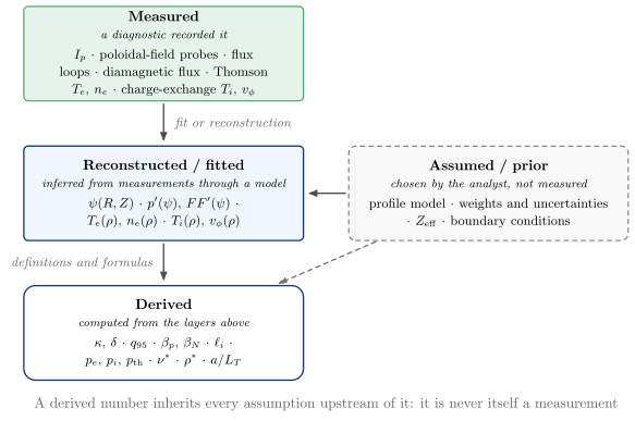
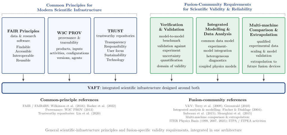
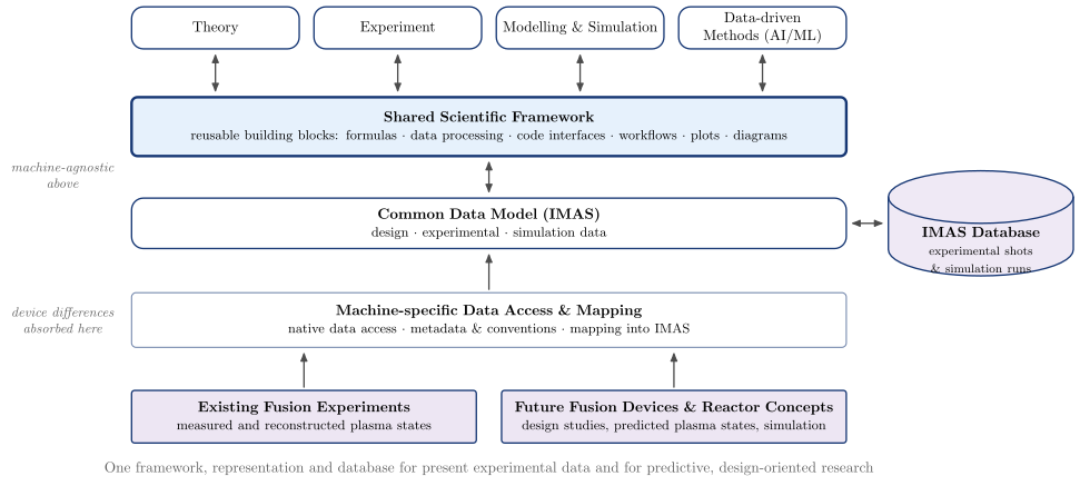
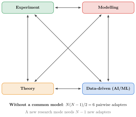
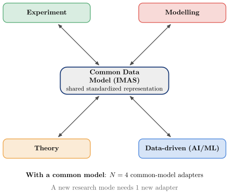
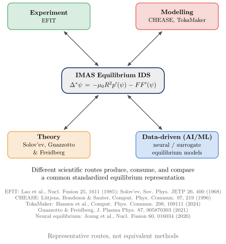
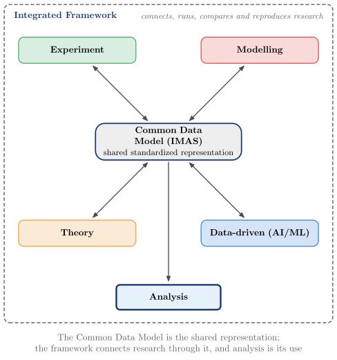
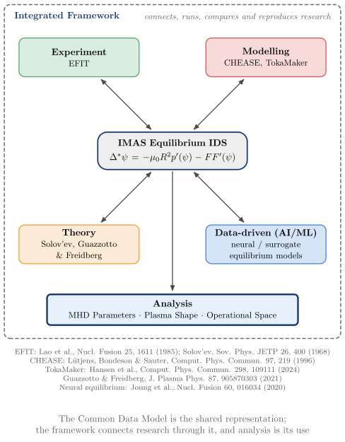
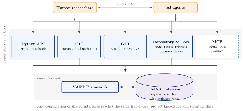
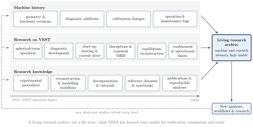
The interoperability figures read as one progression, from data interoperability through scientific integration to infrastructure and implementation. The four nodes of the network and framework figures are research modes, not physics domains; Research domains sets out how the two classifications cross:
- pairwise interfaces,
experiment_modeling_theory_data_network("point_to_point"); - a shared scientific representation,
experiment_modeling_theory_data_network("common_model"); - an integrated scientific framework,
integrated_scientific_framework(), and its equilibrium example,integrated_scientific_framework(domain="equilibrium"); - the broader research infrastructure,
experimental_research_infrastructure()(#1636); - the managed workflow,
scientific_workflow(); - the VEST implementation,
vest_data_platform().
The pillar names are the four README sections.
The diagrams are built from the concept primitives in vaft.diagram._concept: box, connector, band,
and database, a drum drawn as polylines. They use the concept … and connector … styles of the template.
Research infrastructure: four levels of integration, the community and ownership
Why VAFT is built the way it is, in four levels (#1641, #1636, #1638, #1640). Each level is a pair of figures
from one builder: organization="fragmented" draws the problem and organization="integrated" the
architecture that answers it. The pair grammar is shared:
- the fragmented figure draws research paths as dashed silos, joined only by red, dashed ad-hoc links (level 3 is one chain of steps instead, with the evidence each step loses beneath it);
- the integrated figure draws the same entities around the shared layer that replaces those links;
- both carry the level tag at the top left and numbered notes at the bottom, set as columns of text. The fragmented figure lists what goes wrong, each in plain words with its technical term and, where there is one, a reference: ^n plain words (technical term) [reference]. The integrated figure lists what answers each one, under the same number;
- the numbers are cited like footnotes, as a grey superscript after the text they belong to. In the figure they mark where a symptom arises and which part of the architecture answers it, and they run in the order the problem figure cites them.
vaft.diagram.scientific_representation("fragmented")             # level 1, #1641
vaft.diagram.scientific_representation()                         # "integrated" is the default
vaft.diagram.experimental_research_infrastructure("fragmented")  # level 2, #1636
vaft.diagram.scientific_credibility("fragmented")                # level 3, #1638
vaft.diagram.research_modality_architecture("fragmented")        # level 4, #1640
vaft.diagram.fusion_research_ecosystem()                         # #1643, "full" or "presentation"
vaft.diagram.scientific_ownership_architecture()                 # #1645
Read in order, the figures make one argument. A Common Data Model answers the representation problem
(experiment_modeling_theory_data_network). It is not enough on its own: a research infrastructure also
needs a FAIR repository and a research framework. Reproducibility is not enough either: a result also needs
traceable justification. The same science must then serve every researcher, interface and environment. The
managed pipeline is scientific_workflow, and the VEST implementation is vest_data_platform.
| Level | Question | Without | With |
|---|---|---|---|
| 1 Representation | What does this information mean? | One quantity held five ways, and each of four layers fragments on its own: the spoken term (“Ip”, “plasma current”), the stored name (a DAQ channel, a NetCDF variable, a struct field), the structure and the encoding. Stored names are mapped pairwise by hand | Format and structure mappings feed the Common Data Model (IMAS), which owns meaning. Taxonomy, strict aliases and discovery connect researchers and agents to it. Storage and access (local or remote; eager, lazy, partial, cached) sit beside it |
| 2 Infrastructure | How is a state produced, stored and reused? | Five silos, each running source → ad-hoc step → activity with private calibration copies; the reconstruction is copied by hand into other paths | Sources and activities meet only in three complementary capabilities: the Common Data Model, the FAIR Scientific Data Repository and the Research Framework |
| 3 Credibility | Why should this result be trusted for this use? | Locally reasonable steps lose evidence, ending in an apparently precise result. Twelve losses, each with a plain label and the literature term (parametric entanglement, fortuitous agreement, primacy hierarchy, domain of applicability, …) | Provenance, uncertainty and assumptions feed one credibility and traceability structure, which verification, validation and sensitivity examine. The assessment is a profile, not a score, and yields a qualified scientific state |
| 4 Modality & portability | Can every researcher, language and environment use the same science? | The science is copied into a GUI, a notebook, a MATLAB workflow and HPC scripts, and AI gets no capability interface | Sibling interfaces (Python, Jupyter, CLI, GUI, documentation, MCP for agents) sit over shared public APIs and one modular core. Below it are language and runtime interoperability (MATLAB and Julia bindings marked as future) and portable execution. The versioned lifecycle runs beside them |
The figures keep several distinctions visible, and the tests check them:
- HDF5 is a serialization format, not the scientific model. The level-1 figure shows it only as one encoding beside NetCDF, MATLAB files and native outputs, and names no storage service;
- provenance is not validity, numerical verification is not physical applicability, and a surrogate’s training domain is checked apart from its physics model;
- GUI, CLI and MCP are interfaces, never part of the core;
- external solvers keep their own platform limits.
fusion_research_ecosystem asks a different question: who does fusion research, what they do, and which
shared scientific states connect it (#1643). The "full" figure shows research roles a person may combine,
with graduate researchers and learners across every activity. Planning leads to a planned shot and a planned
simulation run. Experiment and simulation are parallel, epistemically distinct producers. Comparison,
validation and synthesis yield qualified states and feed new questions back to planning. Knowledge is
preserved and transferred, and the states serve generic research contexts; only the reference
implementation, VEST, is named. The "presentation" figure is a one-slide projection of the same model,
with shared scientific states feeding experimental planning and operation, physics interpretation and
discovery, and modelling, prediction and validation. Curved arrows show exchange between neighbouring uses;
they do not prescribe a fixed sequence. A test checks that its roles, verbs, states and uses map back to
the detailed figure’s roles, activities and states.
scientific_ownership_architecture shows where scientific logic lives as research software matures (#1645).
Research groups Studies by membership, not by execution order, and neither executes anything. A workflow or
notebook composes computation and matures reusable logic out of itself. Data and the database, and Formula,
Process, Code and learned models, produce results and evidence. Validation interprets that evidence, and an
optional use policy decides what a workflow does about it. The Actor contract is an optional overlay, off
every edge. The graduation rule promotes matured logic by meaning. Computational
layers is the zoomed view of the computation band, and
Scientific architecture uses this figure as VAFT’s
normative architecture.
Related issues: #1090 (the concept family), #1550 (the VEST workflow), #497 (placement of canonical visuals), #248, #252, #1505, #1626-#1629 (provenance, contracts and applicability), #1077, #1165, #1170, #1639, #1642, #669 (ownership, Study, Research, learned models), #1174, #1086, #188, #1423, #1002, #1012, #1013, #1016 (interfaces and runtimes).
References for the terminology in the level-3 and community figures:
- R. Fischer and A. Dinklage, Integrated data analysis of fusion diagnostics by means of the Bayesian probability theory, Rev. Sci. Instrum. 75, 4237 (2004): data inconsistency, parametric entanglement, diagnostic interdependencies, complex error propagation.
- P. W. Terry et al., Validation in fusion research: towards guidelines and best practices, Phys. Plasmas 15, 062503 (2008): qualification, fortuitous agreement, primacy hierarchy.
- M. Greenwald, Verification and validation for magnetic fusion, Phys. Plasmas 17, 058101 (2010).
- W3C, PROV-DM: the PROV data model, W3C Recommendation (2013).
- M. D. Wilkinson et al., The FAIR guiding principles for scientific data management and stewardship, Sci. Data 3, 160018 (2016).
- D. Lin et al., The TRUST principles for digital repositories, Sci. Data 7, 144 (2020).
- F. Imbeaux et al., Design and first applications of the ITER integrated modelling & analysis suite, Nucl. Fusion 55, 123006 (2015).
- ITER Organization, ITER Research Plan within the Staged Approach, ITR-18-03 (2018).
- ITER Physics Basis, Nucl. Fusion 39, 2137 (1999); Progress in the ITER Physics Basis, Nucl. Fusion 47, S1 (2007).
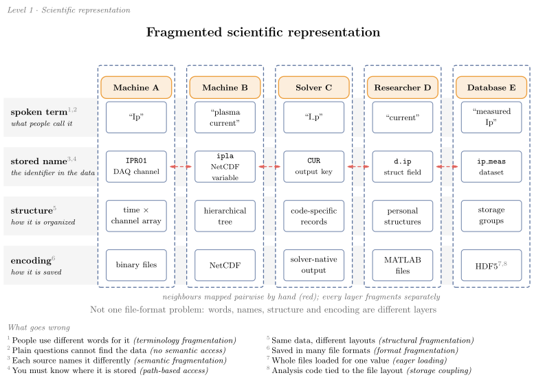
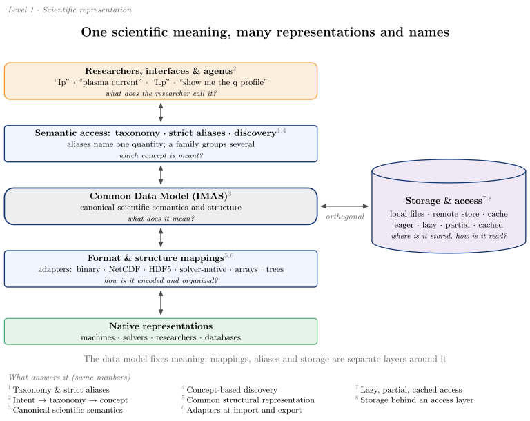
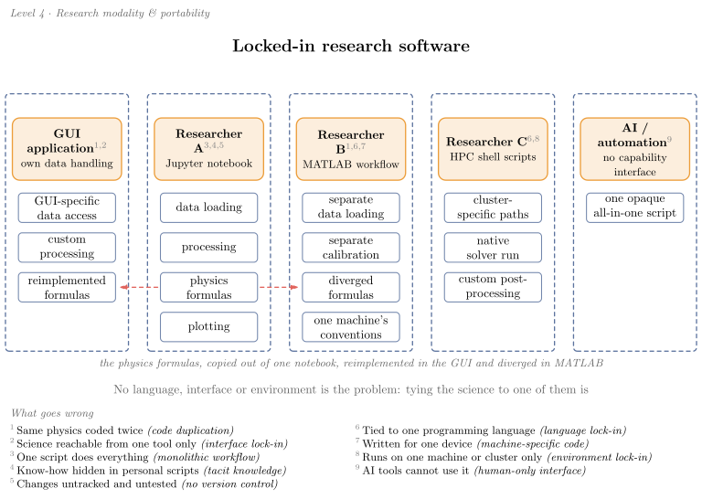
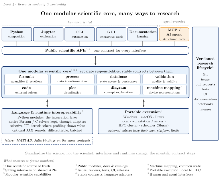
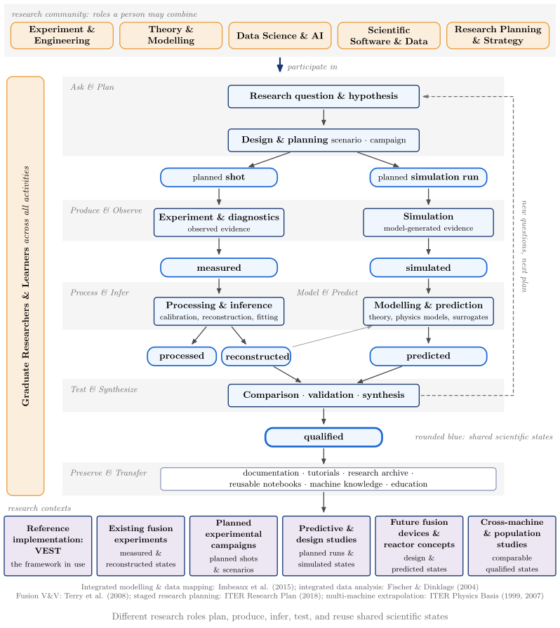
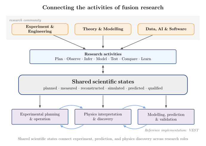
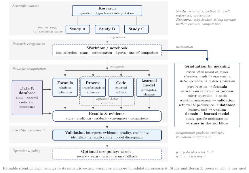
The content is the data at the top of each section of vaft.diagram._research_concepts (INFRA_*,
CREDIBILITY_*, MODALITY_*, REPRESENTATION_*, ECOSYSTEM_*, PRESENTATION_*, OWNERSHIP_*), so a
figure is changed by editing data.
The VEST data platform
The VEST data platform as a database-centred scientific workflow (#1550), laid out as a cross about the
database. The VEST machine, a CAD render packaged with vaft.diagram and embedded in the SVG, sits outside
the platform server and feeds experimental data processing
(the render). A per-shot directory is the hub: reconstruction and physics inference (above) and simulation
(right) read from it and write back to it. Users reach it from below, and the whole runs on Windows,
macOS and Linux, locally or on an HPC cluster. The content is declared in vaft.diagram._platform
(EXPERIMENTAL_PROCESSING, DATABASE_LAYOUT, RECONSTRUCTION, DERIVED_PHYSICS, SIMULATION, ACCESS,
EXECUTION_*), so the figure is updated by editing data. The database technology appears once, as a muted
caption under its title (DATABASE_TECHNOLOGY: IMAS · HDF5 · HSDS); no other backend or workflow-engine names
are drawn.
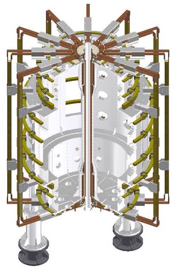
vaft.diagram.vest_data_platform()           # the reference architecture view
vaft.diagram.vest_data_platform_overview()  # five stages, for papers and slides
| Area | Content |
|---|---|
| Experimental data processing | Machine Model & History, Signal Processing, Quality & Validation, Fault & Anomaly Detection, Shot Classification, Event Detection |
| Database | {shot}/: master.h5; experimental files; reconstructed state; physics products; each group open-ended |
| Reconstruction & physics inference | Reconstruction (Eddy Current Model, Magnetic EFIT, Profile Fitting, Plasma Parameter Inference, Kinetic EFIT); Derived Physics (Vacuum Field Proxies, MHD Parameters, Synthetic Diagnostics, Coordinate Conversion, Power Balance) |
| Simulation | Each entry is the concept, with its code or model authors beneath. Equilibrium: Fixed Boundary (CHEASE), Free Boundary (TokaMaker), Analytic GS (Solov’ev · Guazzotto & Freidberg). Stability: Ideal (DCON), Resistive (RDCON). 3D Response & Topology: Plasma Response (GPEC), Field-Line Following (FLARE). Transport: Classical (Braginskii), Neoclassical (NEO / Sauter & Redl), Turbulent (TGLF / CGYRO) |
| Access & analysis | Python API, CLI, GUI, MCP, Documentation; Data Access · Search · Visualization · Comparison · Statistics · Export · Tutorials · Research Archive |
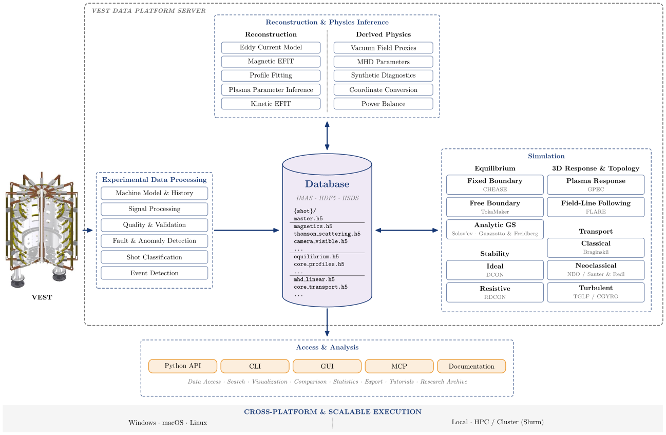
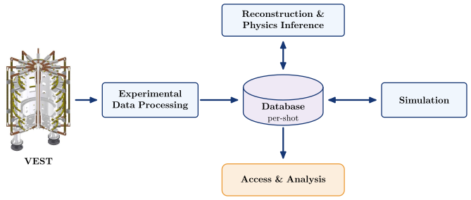
Integrated modeling: knowledge basis, realization, abstraction
A single “analytic / numerical / empirical / data-driven” list mixes three independent questions. These diagrams keep them apart (#1085):
- Knowledge basis: where does the model’s knowledge come from, from first-principles to data-driven?
- Computational realization: how is the model evaluated, from analytical to fully numerical?
- Physical abstraction: at what description level is the system represented, from particle orbits to static equilibrium?
The diagrams then combine the three axes into one space and connect models by typed couplings. They show location and character, not ranking: neither end of an axis is better.
vaft.diagram.knowledge_basis()
vaft.diagram.computational_realization()
vaft.diagram.physical_abstraction()
vaft.diagram.integrated_modeling_space()                 # "fusion", "tearing"
vaft.diagram.integrated_modeling_process()
| Diagram | Concept |
|---|---|
knowledge_basis |
Mechanistic/first-principles, semi-empirical/closure, empirical, data-driven. Physics-informed models (physical constraints with fitted or learned parts) are a bridge over the axis, not one point on it |
computational_realization |
Analytical, semi-analytical, reduced numerical, fully numerical. Learned surrogates are not a rung: they are placed by knowledge basis and role |
physical_abstraction |
Particle/orbit, kinetic, moment/fluid, MHD, equilibrium/static. Each arrow names its reduction: ensemble average, velocity moments + closure, single fluid at low frequency, stationary force balance |
integrated_modeling_space |
Knowledge basis across, realization up. The physical abstraction is shown by the fill colour of each model and repeated in its border pattern, so it survives grayscale. Conceptual and heuristic models (physical picture, cartoon, scaling argument, toy model) are an explanatory layer beside the space, not a fourth axis |
integrated_modeling_process |
Experiment, measurement, processing, inverse model (parameter inference), physical state, forward and data-driven models, prediction, and validation/control, with the eight coupling types of the legend |
Semi-empirical is a knowledge basis: a physical form with fitted coefficients. Semi-analytical is a computational realization: an asymptotic expansion, a Green-function reduction or a quadrature of a closed form. The words look alike but belong to different axes.
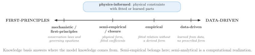
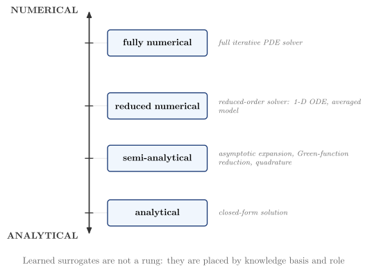
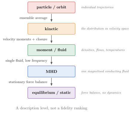
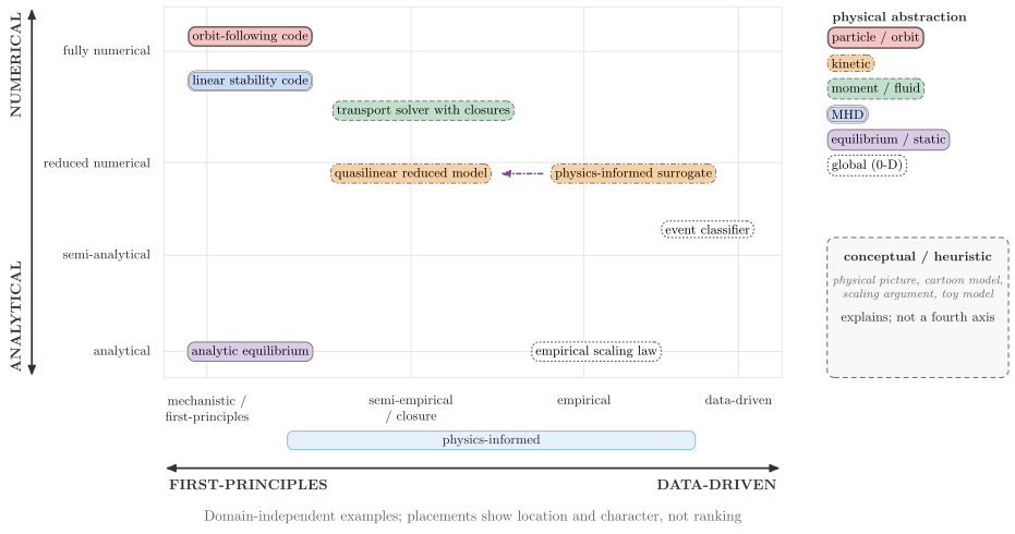
Positions are semantic, not layout. Models with the same knowledge basis share an x and are separated in y. A learned model is not a realization rung. A surrogate takes the y of the model it emulates and is linked to it; a model that emulates nothing, such as a classifier, sits at the rung of its evaluation.
The "fusion" overlay places familiar codes, from Solov’ev, EFIT and CHEASE to TGLF, TRANSP and ASCOT5, with an
empirical confinement scaling, a neural-operator surrogate of TGLF and an event classifier. These placements are
illustrative, not a classification:
- EFIT is an inverse model: it solves the Grad–Shafranov equation numerically inside a fit to measurements.
- TRANSP is mainly used interpretively, so it is also an inverse model.
- DCON integrates the Newcomb ODE, which is a reduced numerical method.
- TGLF is gyro-Landau-fluid approximating gyrokinetics, with a saturation rule fitted to nonlinear gyrokinetic
runs, so it sits at semi-empirical/closure. The
"tearing"variant follows one phenomenon from an island picture in the explanatory layer, through the Rutherford equation, to a nonlinear resistive-MHD simulation.
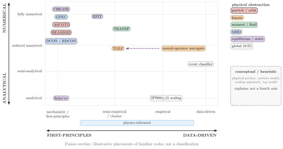
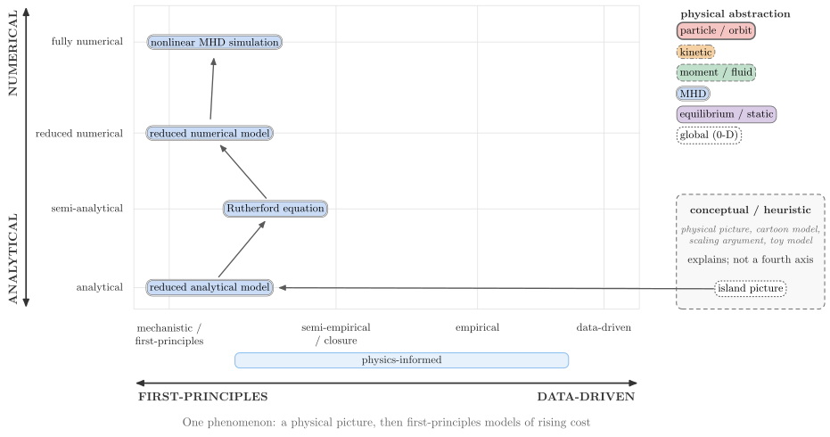
The coupling types are data flow, closure, parameter inference/calibration, surrogate replacement, residual correction, validation/benchmarking, feedback/control and iterative coupling. A coupling is a label on an edge. The data-driven model’s three uses are alternatives: a closure inside the forward model, or a surrogate replacement of it, or a residual correction of its prediction (the hybrid mode). Validation compares the prediction with the processed measurement, and control acts on the experiment.
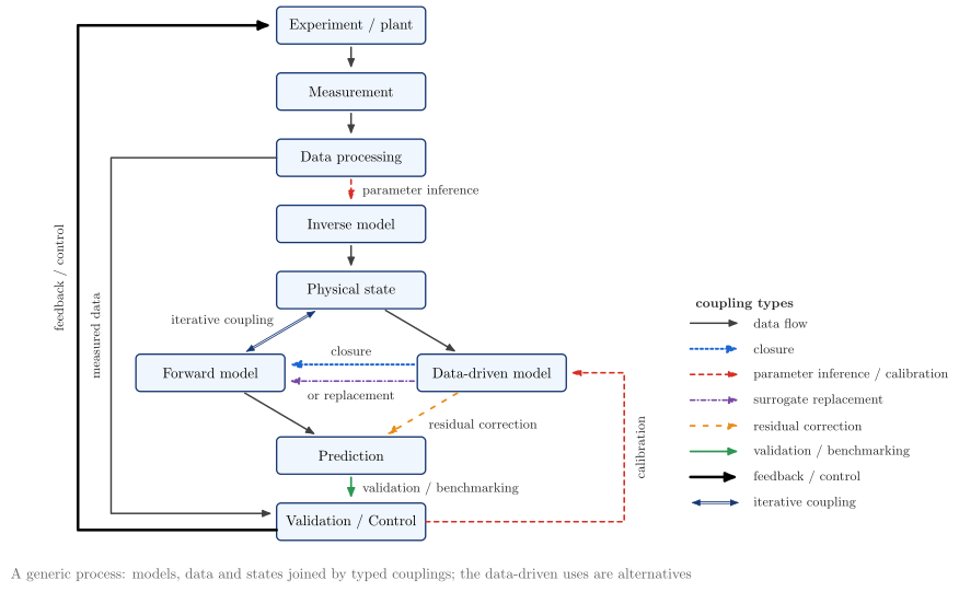
The vocabulary and the example placements are data in vaft.diagram._modeling_schema: the axis stations,
ModelDescriptor, ModelCoupling and the coupling types. They are kept apart from the drawing so that
documentation and provenance tooling can reuse them. They are not a stable public API yet.
Spatial vocabulary: coordinates, geometry, meshes, mappings and topology
Concept-oriented schematics of the spatial ideas VAFT works with, organised by the concept rather than
by a code: a structured grid or a logical mapping is drawn as the numerical idea several equilibrium,
transport and MHD codes share. They need no shot data; vaft.plot draws a particular equilibrium,
mesh or field. vaft.diagram._spatial.SPATIAL_FAMILIES files every builder below by family.
vaft.diagram.tokamak_top_view(cocos=11)
vaft.diagram.cocos_orientation(11)                 # one panel
vaft.diagram.cocos_orientation(range(1, 9))        # one panel per index, one scale
vaft.diagram.machine_and_equilibrium_geometry()
vaft.diagram.structured_rz_grid(n_r=13, n_z=21)
vaft.diagram.geometry_to_mesh()
vaft.diagram.logical_to_physical_mapping()
vaft.diagram.physical_to_flux_mapping()
| Family | Concept | Builder |
|---|---|---|
| coordinate | cylindrical $(R, \phi, Z)$ and toroidal $(r, \theta, \phi)$ | tokamak_torus, tokamak_top_view |
| coordinate | COCOS orientation, generic: $\phi$, $B_\phi$ and $I_p$ (on the magnetic axis) in or out of the page, the sense of $\theta$, the direction $\psi$ increases and its unit; titled by the index and $(\sigma_{B_p}, \sigma_{R\phi Z}, \sigma_{\rho\theta\phi}, \psi)$ | cocos_orientation (signs from vaft.data.cocos.cocos_spec); coordinate choice against COCOS: coordinates_vs_cocos |
| coordinate | flux coordinates $(\psi, \theta, \phi)$ and poloidal angles | flux_coordinates, poloidal_angle_comparison |
| geometry | machine geometry (wall, limiter, coils, passive structure) against equilibrium geometry (axis, surfaces, separatrix, X-point) | machine_and_equilibrium_geometry |
| geometry | limited and diverted equilibria; shaping | limiter_and_diverted_topologies, shaping_family |
| mesh | structured $(R, Z)$ grid with the plasma boundary between nodes | structured_rz_grid |
| mesh | unstructured mesh with region-dependent resolution | geometry_to_mesh |
| mesh | flux-aligned grid; logical $(\xi, \eta) \mapsto (R, Z)$ | logical_to_physical_mapping, sfl_coordinate_grids |
| mapping | measurement at $(R, Z)$ → $\psi$ → $\psi_N$ → $\rho_{\mathrm{tor},N}$ → profile coordinate | physical_to_flux_mapping |
| mapping | geometry → regions → mesh | geometry_to_mesh |
| topology | nested flux surfaces | flux_surfaces |
| topology | X-point and separatrix | x_point, separatrix_lobes |
| topology | magnetic island, stochastic layer | magnetic_island, stochastic_layer |
Conventions shared by every figure: $R$ to the right and $Z$ up in the poloidal plane; $\odot$ out of and
$\otimes$ into the page; the magnetic axis is a filled blue dot, an X-point a cross; the LCFS a black
line, the separatrix blue; the computational boundary dashed; the machine (vessel, limiter, coils) in
black outline, faint where it is shown only for reference; regions shaded plasma blue, vacuum green,
conductor grey; measurements red (outboard) and orange (inboard). The machine and the flux are the toy
free-boundary model of the Grad–Shafranov diagrams, not any device. The sense of $\theta$ differs on
purpose: the cocos_orientation panels draw it as the index fixes it (COCOS 11, $\sigma_{R\phi Z} = +1$
and $\sigma_{\rho\theta\phi} = +1$ with $\phi$ into the page, puts $\theta$ clockwise in the $(R, Z)$ plane
as drawn), while the torus, mesh and mapping figures (tokamak_torus, logical_to_physical_mapping,
sfl_coordinate_grids) are convention-free sketches that use the mathematical angle, counter-clockwise
from the outboard midplane.
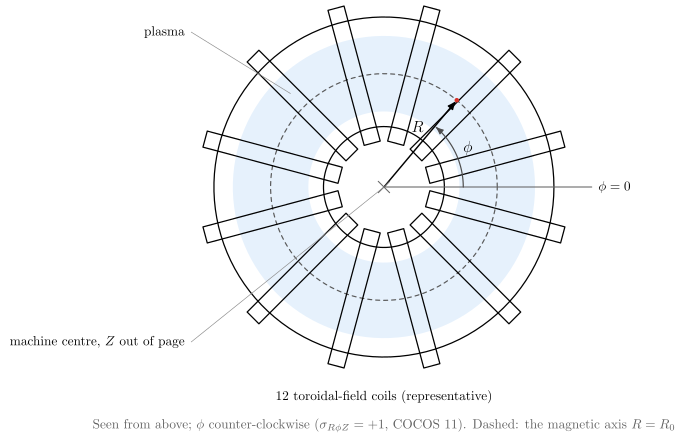
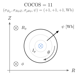
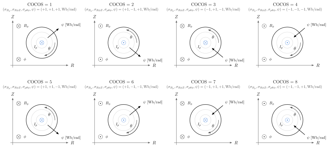
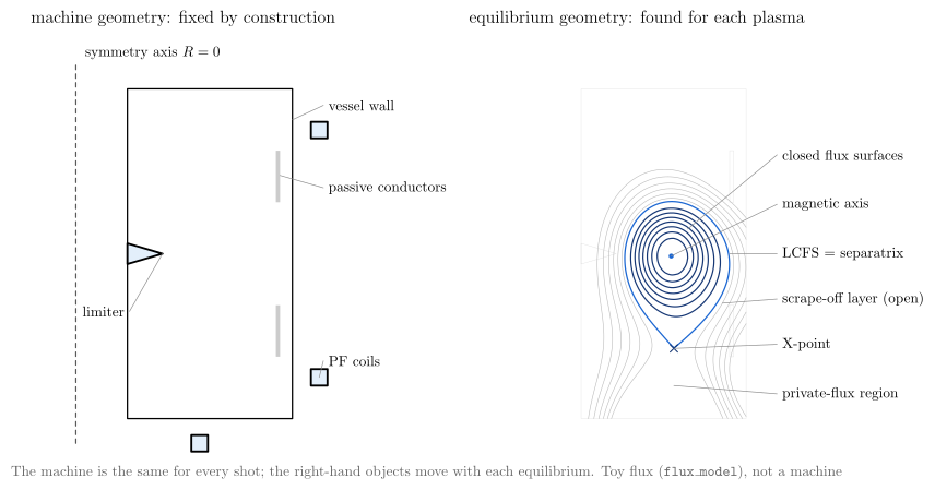
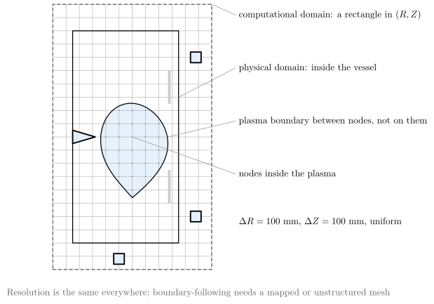
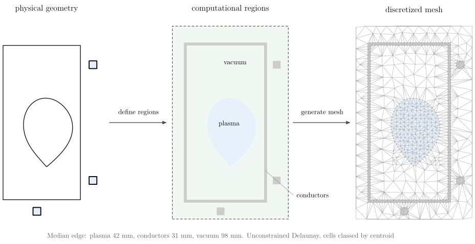
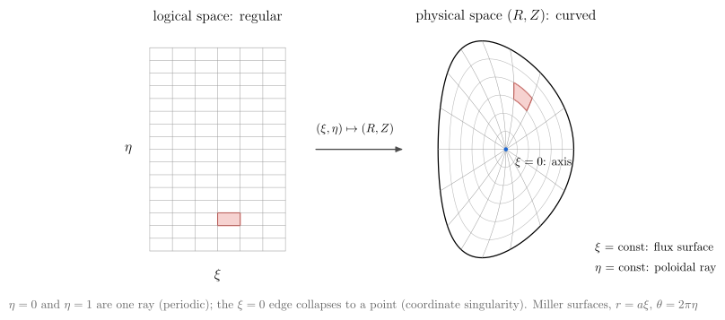
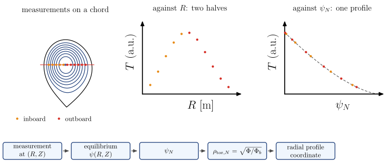
Physics workflows: derivation, inference and solver coupling
The level-2 view below the platform overview (#1585). Each figure is drawn from one declarative
WorkflowSpec (vaft.diagram._workflow); the same record produces the figure and the table under it, and
the tests require every API and equation it names to exist on this tree. The figures follow the current
implementation: where VAFT does not yet implement the physically complete step, or has no IMAS mapping, the
node carries a red IMAS mapping TODO and the workflow lists its follow-up TODOs instead of drawing an
unsupported capability. Node style says how a quantity was obtained:
| Kind | Meaning |
|---|---|
| measured | experimentally observed |
| reconstructed | the solution of an inverse problem |
| derived | computed deterministically from existing state |
| inferred | estimated with a model, prior or closure |
| synthetic (assumption-completed) | completed from an equilibrium and explicit assumptions with no kinetic data; never a measurement |
| model assumption / prior | an assumed value or prior the result depends on; drawn entering from the side |
| model choice / convention | a model choice or convention (basis, sign, conductivity model, mode numbers); drawn from the side |
| machine geometry / static data | static machine data: geometry, Green tables, circuits; drawn from the side |
| code input | a code-specific projection of the canonical state |
| solver / model | an external or internal physical model |
| native result | the solver’s own output, before any mapping |
| standardized IMAS | the IMAS / OMAS representation VAFT stores |
Inputs and outputs carry their representative variables under the label, and standardized nodes their
IMAS path. A step’s equation is drawn inside it: the vaft.formula catalog definition (formula_equation)
where one exists, otherwise a relation restating the expression the named API implements.
vaft.diagram.plasma_parameter_inference()
vaft.diagram.romero_transformer_balance()
vaft.diagram.resistive_zeff_inference()
vaft.diagram.magnetic_efit()
vaft.diagram.kinetic_efit()
vaft.diagram.analytic_mhd_equilibrium()
vaft.diagram.chease_coupling()
vaft.diagram.tokamaker_coupling()
vaft.diagram.dcon_rdcon_stability()
vaft.diagram.gpec_plasma_response()
vaft.diagram.flare_field_line_topology()
vaft.diagram.neo_neoclassical()
vaft.diagram.tglf_cgyro_local_transport()
vaft.diagram.parameter_inference_overview()
vaft.diagram.parameter_inference_dependency_graph()
Plasma parameter inference: ion temperature and species
Measured electron profiles and the equilibrium resolved into an ion temperature, a species mix and the local quantities transport codes read. Each ion-temperature branch is kept apart, and the resolved state is held in memory (ResolvedTransportState), not written back to IMAS.
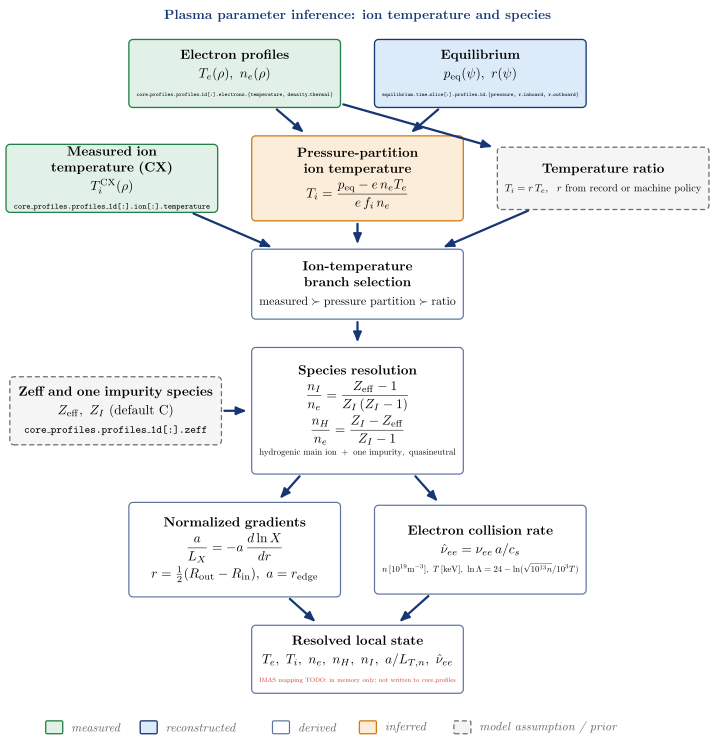
| Node | Kind | Variables | API | IDS |
|---|---|---|---|---|
| Electron profiles | measured | $T_e(\rho),\ n_e(\rho)$ | core_profiles.profiles_1d[:].electrons.{temperature, density_thermal} |
|
| Equilibrium | reconstructed | $p_{\mathrm{eq}}(\psi),\ r(\psi)$ | equilibrium.time_slice[:].profiles_1d.{pressure, r_inboard, r_outboard} |
|
| Measured ion temperature (CX) | measured | $T_i^{\mathrm{CX}}(\rho)$ | core_profiles.profiles_1d[:].ion[:].temperature |
|
| Pressure-partition ion temperature | inferred | vaft.process.kinetic_closure.infer_ti_pressure_partition |
||
| Temperature ratio | model assumption / prior | vaft.machine_mapping.core_profiles.vest_core_profiles_policy |
||
| Ion-temperature branch selection | derived | $\mathrm{measured} \succ \mathrm{pressure\ partition} \succ \mathrm{ratio}$ | vaft.process.transport_state.resolve_transport_state |
|
| Zeff and one impurity species | model assumption / prior (enters Species resolution) | $Z_{\mathrm{eff}},\ Z_I\ (\mathrm{default\ C})$ | core_profiles.profiles_1d[:].zeff |
|
| Species resolution | derived | vaft.code.gacode.inputs.impurity_fractions |
||
| Normalized gradients | derived | vaft.code.gacode.tglf.prepare_tglf_input |
||
| Electron collision rate | derived | vaft.code.gacode.tglf.prepare_tglf_input |
||
| Resolved local state | derived | $T_e,\ T_i,\ n_e,\ n_H,\ n_I,\ a/L_{T,n},\ \hat\nu_{ee}$ | vaft.process.transport_state.resolve_transport_state |
IMAS mapping TODO: in memory only; not written to core_profiles |
Follow-up TODOs (implementation or IMAS mapping):
- The resolved state (T_i choice, n_H, n_I) is not written back to core_profiles.
- Normalized gradients and the GACODE collision rate are computed inside the TGLF input projection, not as vaft.formula definitions.
Plasma resistance from Romero’s transformer balance
The reconstructed boundary flux, plasma current and internal inductance close Romero’s voltage balance; what the inductive part does not explain is the resistive voltage, from which the plasma resistance follows.
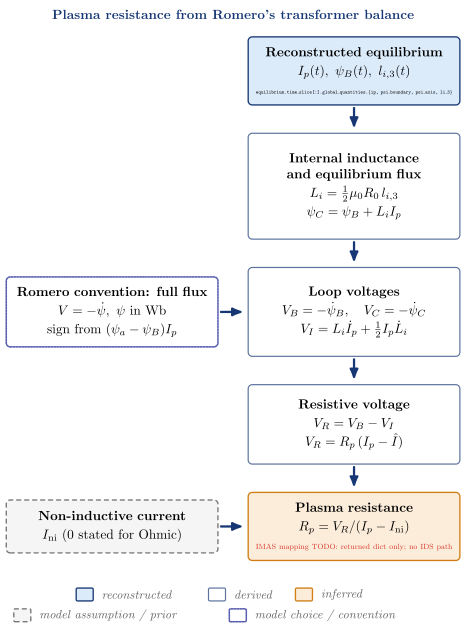
| Node | Kind | Variables | API | IDS |
|---|---|---|---|---|
| Reconstructed equilibrium | reconstructed | $I_p(t),\ \psi_B(t),\ l_{i,3}(t)$ | equilibrium.time_slice[:].global_quantities.{ip, psi_boundary, psi_axis, li_3} |
|
| Romero convention: full flux | model choice / convention (enters Loop voltages) | $V = -\dot\psi,\ \psi\ \mathrm{in\ Wb}, \mathrm{sign\ from}\ (\psi_a - \psi_B)I_p$ | ||
| Internal inductance and equilibrium flux | derived | vaft.omas.process_wrapper.compute_romero_flux_balance_ods |
||
| Loop voltages | derived | vaft.process.equilibrium.romero_flux_balance |
||
| Non-inductive current | model assumption / prior (enters Plasma resistance) | $I_{\mathrm{ni}}\ (0\ \mathrm{stated\ for\ Ohmic})$ | ||
| Resistive voltage | derived | $V_R = V_B - V_I$ | ||
| Plasma resistance | inferred | $R_p = V_R/(I_p - I_{\mathrm{ni}})$ | vaft.omas.process_wrapper.compute_romero_flux_balance_ods |
IMAS mapping TODO: returned dict only; no IDS path |
Follow-up TODOs (implementation or IMAS mapping):
- psi_C is formed as psi_B + L_i I_p from li_3; the current-weighted integral (transformer.current_weighted_flux_from_psi_j_dS) exists but is not used here.
- No IMAS storage for V_B, V_I, V_R or R_p (e.g. summary.global_quantities.v_loop).
Resistively equivalent effective charge
One scalar Zeff over a time window: the effective charge a chosen parallel-conductivity model needs to reproduce the plasma resistance observed through Romero’s balance. It is a model-inferred, resistively equivalent value, not a measured or radially resolved Zeff(rho).
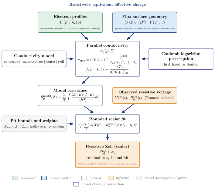
| Node | Kind | Variables | API | IDS |
|---|---|---|---|---|
| Electron profiles | measured | $T_e(\rho),\ n_e(\rho)$ | core_profiles.profiles_1d[:].electrons.{temperature, density} |
|
| Flux-surface geometry | reconstructed | $\langle J!\cdot!B\rangle,\ \langle B^2\rangle,\ V(\psi),\ f_t$ | equilibrium.time_slice[:].profiles_1d.{gm5, volume, f, trapped_fraction} |
|
| Observed resistive voltage | inferred | $V_R^{\mathrm{obs}}(t),\ R_p^{\mathrm{obs}}(t)\ \ (\mathrm{Romero\ balance})$ | vaft.process.resistive_zeff.observed_resistance |
|
| Conductivity model | model choice / convention (enters Parallel conductivity) | $\mathrm{spitzer_nrl \mid sauter_spitzer \mid sauter \mid redl}$ | ||
| Coulomb logarithm prescription | model choice / convention (enters Parallel conductivity) | $\ln\Lambda\ \mathrm{fixed\ or\ Sauter}$ | ||
| Parallel conductivity | derived | $\sigma_\parallel(\rho; Z)$ | vaft.process.resistive_zeff.parallel_conductivity |
|
| Model resistance | derived | vaft.process.resistive_zeff.model_resistance |
||
| Fit bounds and weights | model assumption / prior (enters Bounded scalar fit) | $Z_{\min} \le Z \le Z_{\max}\ (\mathrm{caller\ set}),\ \ w_t\ \mathrm{uniform}$ | ||
| Bounded scalar fit | derived | vaft.process.resistive_zeff.infer_resistive_zeff |
||
| Resistive Zeff (scalar) | inferred | $Z_{\mathrm{eff}}^{\mathrm{res}} \pm \sigma_Z, \mathrm{residual\ rms},\ \mathrm{bound\ hit}$ | IMAS mapping TODO: CSV/JSON product; core_profiles.zeff untouched |
Follow-up TODOs (implementation or IMAS mapping):
- The observed resistance carries no propagated uncertainty (smoothing ‘none’ by default); the Zeff uncertainty is the fit’s sqrt(J/(n-1)/sum w (dV/dZ)^2).
- No IMAS mapping for the scalar resistive Zeff.
Magnetic equilibrium reconstruction (EFIT)
A free-boundary Grad-Shafranov inverse problem: magnetic measurements with their uncertainties, modelled vessel currents and the machine’s Green-function tables constrain a low-order p’ and FF’ basis. EFIT fits; it does not forward-solve.
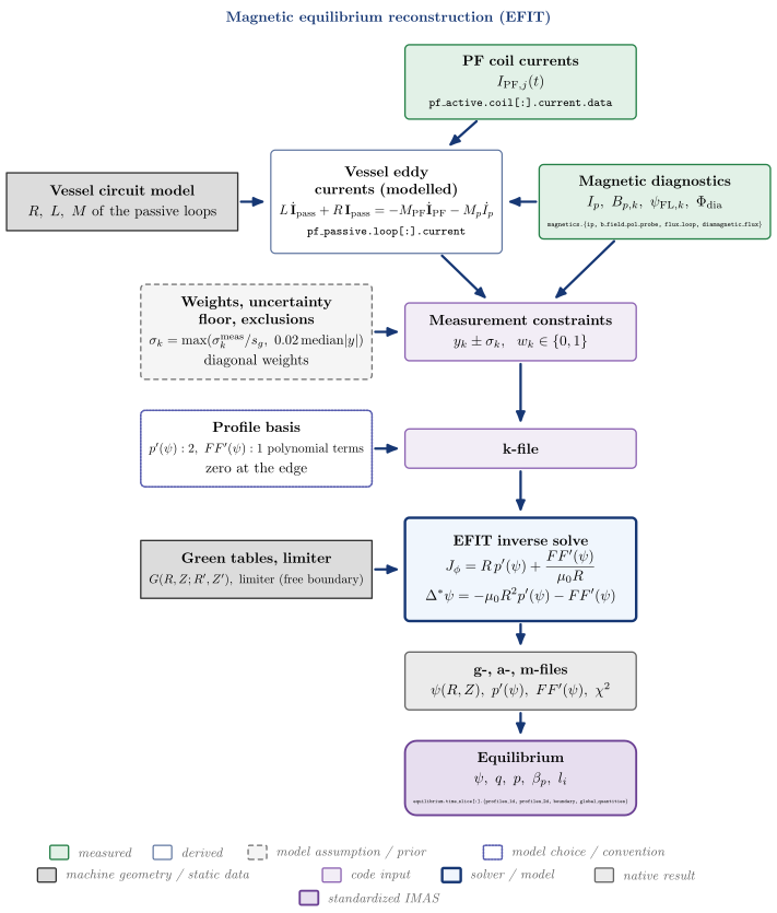
| Node | Kind | Variables | API | IDS |
|---|---|---|---|---|
| PF coil currents | measured | $I_{\mathrm{PF},j}(t)$ | pf_active.coil[:].current.data |
|
| Magnetic diagnostics | measured | $I_p,\ B_{p,k},\ \psi_{\mathrm{FL},k},\ \Phi_{\mathrm{dia}}$ | magnetics.{ip, b_field_pol_probe, flux_loop, diamagnetic_flux} |
|
| Vessel circuit model | machine geometry / static data (enters Vessel eddy currents (modelled)) | $R,\ L,\ M\ \mathrm{of\ the\ passive\ loops}$ | ||
| Vessel eddy currents (modelled) | derived | vaft.process.electromagnetics.solve_eddy_currents |
pf_passive.loop[:].current |
|
| Weights, uncertainty floor, exclusions | model assumption / prior (enters Measurement constraints) | $\sigma_k = \max(\sigma_k^{\mathrm{meas}}/s_g,\ 0.02\,\mathrm{median}|y|), \mathrm{diagonal\ weights}$ | ||
| Measurement constraints | code input | $y_k \pm \sigma_k,\ \ w_k \in {0, 1}$ | vaft.code.efit.generate_constraints_ods |
|
| Profile basis | model choice / convention (enters k-file) | $p’(\psi): 2,\ FF’(\psi): 1\ \mathrm{polynomial\ terms}, \mathrm{zero\ at\ the\ edge}$ | ||
| Green tables, limiter | machine geometry / static data (enters EFIT inverse solve) | $G(R,Z;R’,Z’),\ \mathrm{limiter\ (free\ boundary)}$ | ||
| k-file | code input | vaft.code.efit.prepare_efit_inputs |
||
| EFIT inverse solve | solver / model | vaft.code.efit.run_efit |
||
| g-, a-, m-files | native result | $\psi(R,Z),\ p’(\psi),\ FF’(\psi),\ \chi^2$ | vaft.code.efit.collect_efit_outputs |
|
| Equilibrium | standardized IMAS | $\psi,\ q,\ p,\ \beta_p,\ l_i$ | vaft.code.efit.gfile_to_omas |
equilibrium.time_slice[:].{profiles_1d, profiles_2d, boundary, global_quantities} |
Follow-up TODOs (implementation or IMAS mapping):
- Vessel currents are modelled from a circuit driven by measured PF currents and I_p filaments, not fitted (IFITVS=0 by default); no flux loop constrains them.
- Measurement weighting is diagonal; no covariance enters EFIT.
- Native k/g/a/m files are recorded only by path and hash under equilibrium.code.parameters.
Kinetically constrained equilibrium reconstruction
The magnetic constraints plus a kinetic pressure profile: Thomson T_e, n_e and a measured or ratio-assumed T_i give pressure points with propagated uncertainty, placed in real space so EFIT maps them to psi on its own solution.
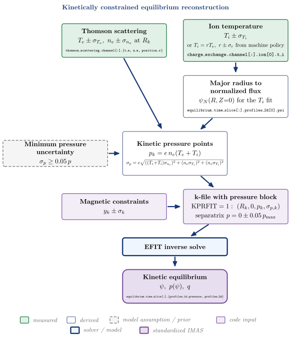
| Node | Kind | Variables | API | IDS |
|---|---|---|---|---|
| Thomson scattering | measured | $T_e \pm \sigma_{T_e},\ n_e \pm \sigma_{n_e}\ \mathrm{at}\ R_k$ | thomson_scattering.channel[:].{t_e, n_e, position.r} |
|
| Ion temperature | measured | $T_i \pm \sigma_{T_i}, \mathrm{or}\ T_i = rT_e,\ r \pm \sigma_r\ \mathrm{from\ machine\ policy}$ | charge_exchange.channel[:].ion[0].t_i |
|
| Major radius to normalized flux | derived | $\psi_N(R, Z{=}0)\ \mathrm{for\ the}\ T_i\ \mathrm{fit}$ | equilibrium.time_slice[:].profiles_2d[0].psi |
|
| Kinetic pressure points | derived | vaft.code.efit.kinetic_pressure_points |
||
| Minimum pressure uncertainty | model assumption / prior (enters Kinetic pressure points) | $\sigma_p \ge 0.05\,p$ | ||
| Magnetic constraints | code input | $y_k \pm \sigma_k$ | vaft.code.efit.generate_constraints_ods |
|
| k-file with pressure block | code input | $\mathrm{KPRFIT}=1:\ (R_k, 0, p_k, \sigma_{p,k}), \mathrm{separatrix}\ p = 0 \pm 0.05\,p_{\max}$ | vaft.code.efit.inject_pressure_constraint |
|
| EFIT inverse solve | solver / model | vaft.code.efit.run_kinetic_efit |
||
| Kinetic equilibrium | standardized IMAS | $\psi,\ p(\psi),\ q$ | vaft.code.efit.run_kinetic_chain |
equilibrium.time_slice[:].{profiles_1d.pressure, profiles_2d} |
Follow-up TODOs (implementation or IMAS mapping):
- Pressure assumes one ion species with n_i = n_e: no impurity dilution or Zeff enters p_kin.
- The pressure points and the Ip scale run_kinetic_efit settles on are not stored in IMAS (manifest only); the work directory with the k-file is deleted.
- Single pass against the magnetic equilibrium: no kinetic <-> equilibrium iteration.
Analytic MHD equilibrium models
Two uses of closed-form Grad-Shafranov solutions. Forward generation builds an equilibrium from shape parameters and a profile class; fitting projects a reconstructed equilibrium onto a Solov’ev basis and reports how well it is represented.
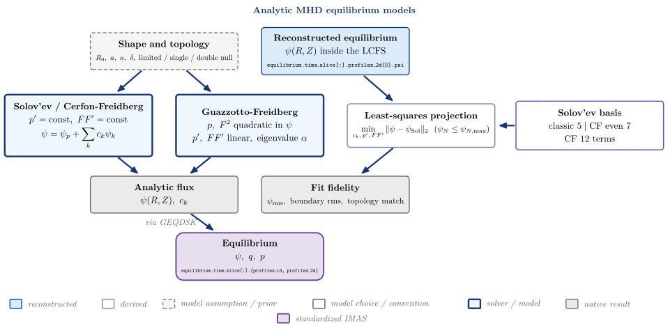
| Node | Kind | Variables | API | IDS |
|---|---|---|---|---|
| Shape and topology | model assumption / prior | $R_0,\ a,\ \kappa,\ \delta,\ \mathrm{limited\ /\ single\ /\ double\ null}$ | ||
| Reconstructed equilibrium | reconstructed | $\psi(R,Z)\ \mathrm{inside\ the\ LCFS}$ | equilibrium.time_slice[:].profiles_2d[0].psi |
|
| Solov’ev / Cerfon-Freidberg | solver / model | vaft.process.solve_solovev_constraints |
||
| Guazzotto-Freidberg | solver / model | vaft.process.solve_guazzotto_freidberg |
||
| Solov’ev basis | model choice / convention (enters Least-squares projection) | $\mathrm{classic}\ 5 \mid \mathrm{CF\ even}\ 7, \mathrm{CF}\ 12\ \mathrm{terms}$ | ||
| Least-squares projection | derived | vaft.process.fit_solovev |
||
| Analytic flux | native result | $\psi(R,Z),\ c_k$ | ||
| Fit fidelity | native result | $\psi_{\mathrm{rms}},\ \mathrm{boundary\ rms},\ \mathrm{topology\ match}$ | ||
| Equilibrium | standardized IMAS | $\psi,\ q,\ p$ | vaft.data.eqdsk.to_omas |
equilibrium.time_slice[:].{profiles_1d, profiles_2d} |
Follow-up TODOs (implementation or IMAS mapping):
- No direct ODS writer: forward results reach IMAS through EquilibriumData -> GEQDSK -> to_omas.
- Fit results (SolovevFit) are not written to IMAS.
Fixed-boundary equilibrium refinement (CHEASE)
A reconstructed boundary and profiles re-solved at fixed boundary; the COCOS transform into and out of CHEASE is explicit.
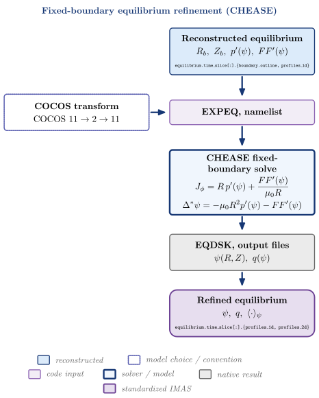
| Node | Kind | Variables | API | IDS |
|---|---|---|---|---|
| Reconstructed equilibrium | reconstructed | $R_b,\ Z_b,\ p’(\psi),\ FF’(\psi)$ | equilibrium.time_slice[:].{boundary.outline, profiles_1d} |
|
| COCOS transform | model choice / convention (enters EXPEQ, namelist) | $\mathrm{COCOS}\ 11 \to 2 \to 11$ | ||
| EXPEQ, namelist | code input | vaft.code.chease.prepare_chease_inputs |
||
| CHEASE fixed-boundary solve | solver / model | vaft.code.chease.run_chease |
||
| EQDSK, output files | native result | $\psi(R,Z),\ q(\psi)$ | vaft.code.chease.collect_chease_outputs |
|
| Refined equilibrium | standardized IMAS | $\psi,\ q,\ \langle\cdot\rangle_\psi$ | vaft.code.chease.refine_equilibrium |
equilibrium.time_slice[:].{profiles_1d, profiles_2d} |
Free-boundary equilibrium (TokaMaker)
Machine geometry, measured coil currents and power-law profile shapes solved at free boundary on a finite-element mesh; the plasma boundary is part of the solution.
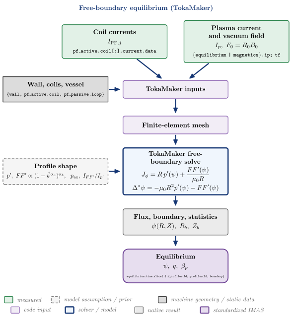
| Node | Kind | Variables | API | IDS |
|---|---|---|---|---|
| Coil currents | measured | $I_{\mathrm{PF},j}$ | pf_active.coil[:].current.data |
|
| Plasma current and vacuum field | measured | $I_p,\ F_0 = R_0 B_0$ | {equilibrium | magnetics}.ip; tf |
|
| Wall, coils, vessel | machine geometry / static data (enters TokaMaker inputs) | {wall, pf_active.coil, pf_passive.loop} |
||
| TokaMaker inputs | code input | vaft.code.tokamaker.prepare_tokamaker_inputs |
||
| Finite-element mesh | code input | vaft.code.tokamaker.build_tokamaker_mesh |
||
| Profile shape | model assumption / prior (enters TokaMaker free-boundary solve) | $p’,\ FF’ \propto (1-\hat\psi^{\alpha_a})^{\alpha_b},\ \ p_{\mathrm{ax}},\ I_{FF’}/I_{p’}$ | ||
| TokaMaker free-boundary solve | solver / model | vaft.code.tokamaker.run_tokamaker |
||
| Flux, boundary, statistics | native result | $\psi(R,Z),\ R_b,\ Z_b$ | vaft.code.tokamaker.collect_tokamaker_outputs |
|
| Equilibrium | standardized IMAS | $\psi,\ q,\ \beta_p$ | equilibrium.time_slice[:].{profiles_1d, profiles_2d, boundary} |
Ideal and resistive MHD stability (DCON / RDCON)
An equilibrium tested for ideal stability (DCON energy principle) and for tearing (RDCON matching at the rational surfaces); the solver-native energies and Delta-prime come before any verdict.
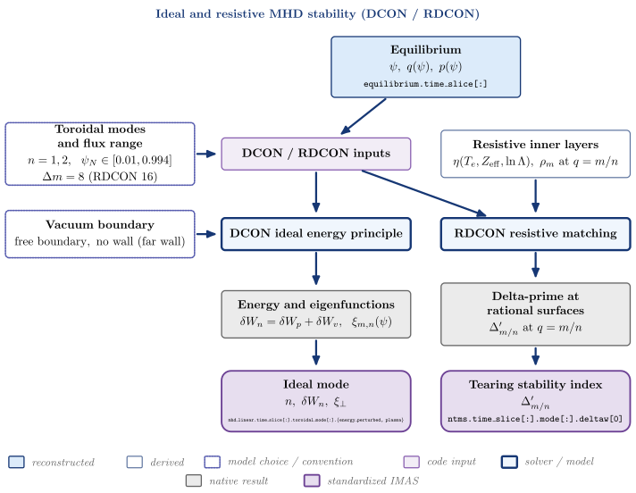
| Node | Kind | Variables | API | IDS |
|---|---|---|---|---|
| Equilibrium | reconstructed | $\psi,\ q(\psi),\ p(\psi)$ | equilibrium.time_slice[:] |
|
| Toroidal modes and flux range | model choice / convention (enters DCON / RDCON inputs) | $n = 1, 2,\ \ \psi_N \in [0.01, 0.994], \Delta m = 8\ (\mathrm{RDCON}\ 16)$ | ||
| DCON / RDCON inputs | code input | vaft.code.gpec.prepare_gpec_suite_case |
||
| Vacuum boundary | model choice / convention (enters DCON ideal energy principle) | $\mathrm{free\ boundary,\ no\ wall\ (far\ wall)}$ | ||
| Resistive inner layers | derived | $\eta(T_e, Z_{\mathrm{eff}}, \ln\Lambda),\ \rho_m\ \mathrm{at}\ q = m/n$ | vaft.code.gpec._solvers.write_rmatch_resistive_layers |
|
| DCON ideal energy principle | solver / model | vaft.code.gpec.run_gpec_suite_case |
||
| RDCON resistive matching | solver / model | vaft.code.gpec.run_gpec_suite_case |
||
| Energy and eigenfunctions | native result | $\delta W_n = \delta W_p + \delta W_v,\ \ \xi_{m,n}(\psi)$ | vaft.code.gpec.read_dcon_output |
|
| Delta-prime at rational surfaces | native result | $\Delta’_{m/n}\ \mathrm{at}\ q = m/n$ | vaft.code.gpec.read_pest3_matching_output |
|
| Ideal mode | standardized IMAS | $n,\ \delta W_n,\ \xi_\perp$ | mhd_linear.time_slice[:].toroidal_mode[:].{energy_perturbed, plasma} |
|
| Tearing stability index | standardized IMAS | $\Delta’_{m/n}$ | ntms.time_slice[:].mode[:].deltaw[0] |
Follow-up TODOs (implementation or IMAS mapping):
- energy_perturbed carries the DCON-normalised total delta W, not joules; the plasma/vacuum split and the full Delta-prime matrices stay native.
- Wall position, qlow and delta_mlow/high come from the packaged templates, not from VAFT options.
Ideal plasma response to 3-D fields (GPEC)
An applied non-axisymmetric coil field and the plasma’s ideal response to it: coil geometry is machine data, the excitation is prescribed, and the total, plasma and resonant fields are kept apart.
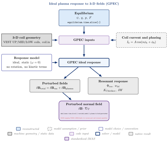
| Node | Kind | Variables | API | IDS |
|---|---|---|---|---|
| Equilibrium | reconstructed | $\psi,\ q,\ p,\ F$ | equilibrium.time_slice[:] |
|
| 3-D coil geometry | machine geometry / static data (enters GPEC inputs) | $\mathrm{VEST\ UP/MID/LOW\ coils,\ coil.in}$ | ||
| Coil current and phasing | model assumption / prior (enters GPEC inputs) | vaft.machine_mapping.coils_non_axisymmetric_geometry.CoilExcitation.from_mode |
||
| GPEC inputs | code input | vaft.code.gpec.prepare_gpec_suite_case |
||
| Response model | model choice / convention (enters GPEC ideal response) | $\mathrm{ideal,\ static}\ (\omega = 0), \mathrm{no\ rotation,\ no\ kinetic\ terms}$ | ||
| GPEC ideal response | solver / model | vaft.code.gpec.run_gpec_suite_case |
||
| Perturbed fields | native result | $\delta\mathbf B_{\mathrm{total}} = \delta\mathbf B_{\mathrm{vac}} + \delta\mathbf B_{\mathrm{plasma}}$ | vaft.code.gpec.read_gpec_netcdf |
|
| Resonant response | native result | $\Phi_{\mathrm{res}},\ w_{\mathrm{isl}}, K_{\mathrm{Chirikov}},\ \delta W$ | vaft.code.gpec.read_gpec_netcdf |
|
| Perturbed normal field | standardized IMAS | $\delta\mathbf B\cdot\nabla\psi$ | mhd_linear.time_slice[:].toroidal_mode[:].plasma.b_field_perturbed; IMAS mapping TODO: dB(R,Z,phi), its vacuum part and resonant quantities |
Follow-up TODOs (implementation or IMAS mapping):
- GPEC returns total and plasma fields; the vacuum part (total minus plasma) is not computed by any mapping.
- No frequency, rotation or kinetic response inputs: the response is ideal and static.
- Energies go to code.parameters; resonant quantities and cylindrical fields are not mapped.
Magnetic field-line topology (FLARE)
Field lines traced through the axisymmetric background plus the 3-D perturbation: Poincare maps, connection lengths and strike-point footprints are the native products; a heat load needs an explicit model, here a relative proxy.
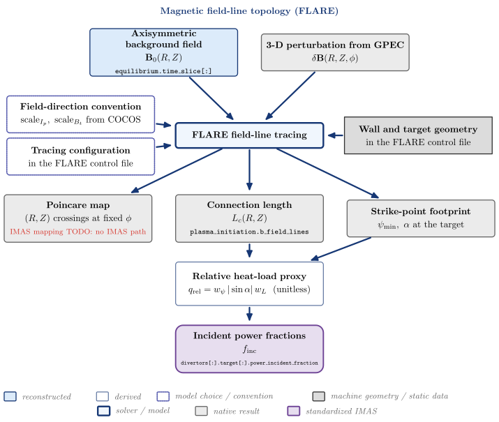
| Node | Kind | Variables | API | IDS |
|---|---|---|---|---|
| Axisymmetric background field | reconstructed | $\mathbf B_0(R,Z)$ | equilibrium.time_slice[:] |
|
| 3-D perturbation from GPEC | native result | $\delta\mathbf B(R,Z,\phi)$ | vaft.code.flare.write_helicity_flipped_field |
|
| Field-direction convention | model choice / convention (enters FLARE field-line tracing) | $\mathrm{scale}{I_p},\ \mathrm{scale}{B_t}\ \mathrm{from\ COCOS}$ | vaft.code.flare.flare_equilibrium_scales |
|
| Wall and target geometry | machine geometry / static data (enters FLARE field-line tracing) | $\mathrm{in\ the\ FLARE\ control\ file}$ | ||
| Tracing configuration | model choice / convention (enters FLARE field-line tracing) | $\mathrm{in\ the\ FLARE\ control\ file}$ | ||
| FLARE field-line tracing | solver / model | vaft.code.flare.run_flare |
||
| Poincare map | native result | $(R, Z)\ \mathrm{crossings\ at\ fixed}\ \phi$ | vaft.data.flare_products.read_flare_product |
IMAS mapping TODO: no IMAS path |
| Connection length | native result | $L_c(R,Z)$ | plasma_initiation.b_field_lines |
|
| Strike-point footprint | native result | $\psi_{\min},\ \alpha\ \mathrm{at\ the\ target}$ | ||
| Relative heat-load proxy | derived | vaft.process.field_line_topology.footprint_heat_load_proxy |
||
| Incident power fractions | standardized IMAS | $f_{\mathrm{inc}}$ | divertors[:].target[:].power_incident_fraction |
Follow-up TODOs (implementation or IMAS mapping):
- Wall/target geometry and tracing settings live in the user’s FLARE control file, not in VAFT.
- No island width or stochasticity metric is computed from FLARE output (GPEC’s Chirikov K is the only one in VAFT).
- The heat load is a relative proxy; no parallel-transport or q_perp model is implemented.
Neoclassical transport: closed-form fits and drift-kinetic solution
The same resolved local state through the Sauter and Redl fits and the drift-kinetic solver NEO, so the two can be compared at one state.
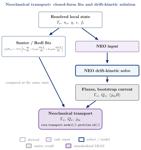
| Node | Kind | Variables | API | IDS |
|---|---|---|---|---|
| Resolved local state | derived | $T_s,\ n_s,\ q,\ \epsilon,\ f_t$ | vaft.process.transport_state.resolve_transport_state |
|
| Sauter / Redl fits | derived | vaft.formula.neoclassical.redl_bootstrap_current |
||
| NEO input | code input | vaft.code.gacode.neo.prepare_neo_case |
||
| NEO drift-kinetic solve | solver / model | vaft.code.gacode.neo.run_neo |
||
| Fluxes, bootstrap current | native result | $\Gamma_s,\ Q_s,\ \langle j_{\mathrm{bs}}B\rangle$ | vaft.code.gacode.neo.collect_neo_outputs |
|
| Neoclassical transport | standardized IMAS | $\Gamma_s,\ Q_s,\ j_{\mathrm{bs}}$ | core_transport.model[:].profiles_1d[:] |
Local turbulent transport: quasilinear and gyrokinetic
One local gyrokinetic state projected into TGLF (quasilinear) and CGYRO (local delta-f, linear or nonlinear); their outputs are different physical objects and are kept apart.
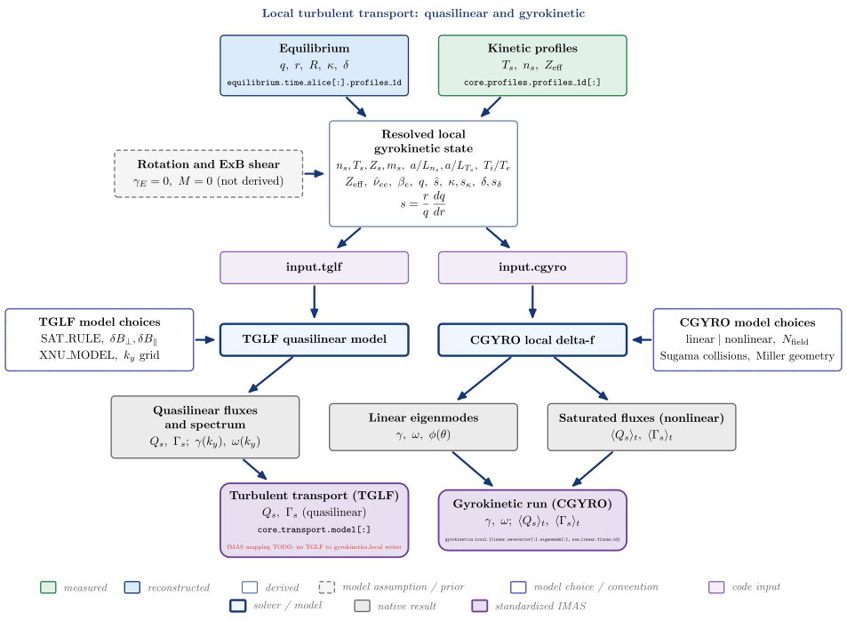
| Node | Kind | Variables | API | IDS |
|---|---|---|---|---|
| Equilibrium | reconstructed | $q,\ r,\ R,\ \kappa,\ \delta$ | equilibrium.time_slice[:].profiles_1d |
|
| Kinetic profiles | measured | $T_s,\ n_s,\ Z_{\mathrm{eff}}$ | core_profiles.profiles_1d[:] |
|
| Resolved local gyrokinetic state | derived | $n_s, T_s, Z_s, m_s,\ a/L_{n_s}, a/L_{T_s},\ T_i/T_e, Z_{\mathrm{eff}},\ \hat\nu_{ee},\ \beta_e,\ q,\ \hat s,\ \kappa, s_\kappa,\ \delta, s_\delta$ | vaft.process.transport_state.resolve_transport_state |
|
| Rotation and ExB shear | model assumption / prior (enters Resolved local gyrokinetic state) | $\gamma_E = 0,\ M = 0\ (\mathrm{not\ derived})$ | ||
| input.tglf | code input | vaft.code.gacode.tglf.prepare_tglf_input |
||
| input.cgyro | code input | vaft.code.gacode.cgyro.prepare_cgyro_input |
||
| TGLF model choices | model choice / convention (enters TGLF quasilinear model) | $\mathrm{SAT_RULE},\ \delta B_\perp, \delta B_\parallel, \mathrm{XNU_MODEL},\ k_y\ \mathrm{grid}$ | ||
| TGLF quasilinear model | solver / model | vaft.code.gacode.tglf.run_tglf |
||
| CGYRO local delta-f | solver / model | vaft.code.gacode.cgyro.run_cgyro |
||
| CGYRO model choices | model choice / convention (enters CGYRO local delta-f) | $\mathrm{linear \mid nonlinear},\ N_{\mathrm{field}}, \mathrm{Sugama\ collisions},\ \mathrm{Miller\ geometry}$ | ||
| Quasilinear fluxes and spectrum | native result | $Q_s,\ \Gamma_s;\ \gamma(k_y),\ \omega(k_y)$ | vaft.code.gacode.tglf.collect_tglf_outputs |
|
| Linear eigenmodes | native result | $\gamma,\ \omega,\ \phi(\theta)$ | vaft.code.gacode.cgyro.collect_cgyro_outputs |
|
| Saturated fluxes (nonlinear) | native result | $\langle Q_s\rangle_t,\ \langle\Gamma_s\rangle_t$ | vaft.code.gacode.cgyro.collect_cgyro_outputs |
|
| Turbulent transport (TGLF) | standardized IMAS | $Q_s,\ \Gamma_s\ \mathrm{(quasilinear)}$ | vaft.machine_mapping.turbulence.core_transport_from_tglf |
core_transport.model[:]; IMAS mapping TODO: no TGLF to gyrokinetics_local writer |
| Gyrokinetic run (CGYRO) | standardized IMAS | $\gamma,\ \omega;\ \langle Q_s\rangle_t,\ \langle\Gamma_s\rangle_t$ | vaft.machine_mapping.gyrokinetics.gyrokinetics_local_from_cgyro |
gyrokinetics_local.{linear.wavevector[:].eigenmode[:], non_linear.fluxes_1d} |
Follow-up TODOs (implementation or IMAS mapping):
- Rotation and ExB shear are zero in both projections (TGLF VEXB_SHEAR, CGYRO GAMMA_E, MACH): their derivation from data is not implemented (#553).
- Squareness zeta enters as 0 (VEST equilibria carry no squareness); Z_EFF is not written to input.cgyro by design: CGYRO recomputes it from the species list (Z_EFF_METHOD=2).
- No implemented local-gyrokinetic validity criterion (rho*): compare_with_oracle checks only the input translation against CGYRO’s own projection.
- No TGLF to gyrokinetics_local mapping.
Plasma parameter inference: completing the kinetic profiles
Where inference sits: diagnostics and the equilibrium give reconstructed but incomplete kinetic profiles; explicit assumptions and the closures VAFT implements complete them, and every completed quantity keeps its origin on the way to simulation.
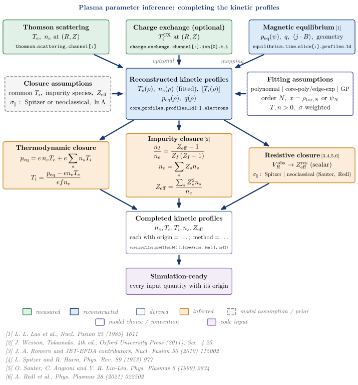
| Node | Kind | Variables | API | IDS |
|---|---|---|---|---|
| Thomson scattering | measured | $T_e,\ n_e\ \mathrm{at}\ (R, Z)$ | thomson_scattering.channel[:] |
|
| Charge exchange (optional) | measured | $T_i^{\mathrm{CX}}\ \mathrm{at}\ (R, Z)$ | charge_exchange.channel[:].ion[0].t_i |
|
| Magnetic equilibrium | reconstructed | $p_{\mathrm{eq}}(\psi),\ q,\ \langle j\cdot B\rangle,\ \mathrm{geometry}$ | equilibrium.time_slice[:].profiles_1d |
|
| Reconstructed kinetic profiles | reconstructed | $T_e(\rho),\ n_e(\rho)\ (\mathrm{fitted}),\ [T_i(\rho)], p_{\mathrm{eq}}(\rho),\ q(\rho)$ | core_profiles.profiles_1d[:].electrons |
|
| Fitting assumptions | model choice / convention (enters Reconstructed kinetic profiles) | $\mathrm{polynomial\ |\ core\text{-}poly/edge\text{-}exp\ |\ GP}, \mathrm{order}\ N,\ x = \rho_{\mathrm{tor},N}\ \mathrm{or}\ \psi_N, T, n > 0,\ \sigma\text{-}\mathrm{weighted}$ | vaft.process.profile.profile_fitting_thomson_scattering |
|
| Closure assumptions | model assumption / prior (enters Reconstructed kinetic profiles) | $\mathrm{common}\ T_i,\ \mathrm{impurity\ species},\ Z_{\mathrm{eff}}, \sigma_\parallel:\ \mathrm{Spitzer\ or\ neoclassical},\ \ln\Lambda$ | ||
| Thermodynamic closure | inferred | vaft.process.kinetic_closure.infer_ti_pressure_partition |
||
| Impurity closure | inferred | vaft.process.impurity.resolve_impurity_composition |
||
| Resistive closure | inferred | $V_R^{\mathrm{obs}} \to Z_{\mathrm{eff}}^{\mathrm{res}}\ (\mathrm{scalar}), \sigma_\parallel:\ \mathrm{Spitzer\ |\ neoclassical\ (Sauter,\ Redl)}$ | vaft.process.resistive_zeff.infer_resistive_zeff |
|
| Completed kinetic profiles | derived | $n_e, T_e, T_i, n_s, Z_{\mathrm{eff}}, \mathrm{each\ with\ origin=\ldots;\ method=\ldots}$ | core_profiles.profiles_1d[:].{electrons, ion[:], zeff} |
|
| Simulation-ready | code input | $\mathrm{every\ input\ quantity\ with\ its\ origin}$ |
References:
- L. L. Lao et al., Nucl. Fusion 25 (1985) 1611
- J. Wesson, Tokamaks, 4th ed., Oxford University Press (2011), Sec. 4.25
- J. A. Romero and JET-EFDA contributors, Nucl. Fusion 50 (2010) 115002
- L. Spitzer and R. Harm, Phys. Rev. 89 (1953) 977
- O. Sauter, C. Angioni and Y. R. Lin-Liu, Phys. Plasmas 6 (1999) 2834
- A. Redl et al., Phys. Plasmas 28 (2021) 022502
Follow-up TODOs (implementation or IMAS mapping):
- Atomic-model-constrained Z_eff(rho) (transient charge states projected through the resistive closure) is on develop as resolve_radial_composition(normalization=’resistive_closure’) (#1565, #1566, PR #1659); this diagram still draws the scalar resistive closure only.
- Rotation, E_r and the ExB shear are not inferred: downstream codes receive gamma_E = 0 as an explicit assumption (#553).
- Provenance is recorded per quantity where it exists (core_profiles origin=…; method=… records for composition, the T_i result’s origin/method fields); there is no single runtime provenance object, by design (#1601 is documentation-first).
Inferred quantities depend on inferred quantities
Provenance propagates: a composition assumption fixes the ion densities, which set the pressure-partition T_i, whose gradients reach the gyrokinetic input beside an assumed zero ExB shear. Every link below the measurements carries the assumptions above it.
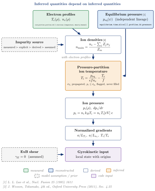
| Node | Kind | Variables | API | IDS |
|---|---|---|---|---|
| Electron profiles | measured | $T_e(\rho),\ n_e(\rho)$ | core_profiles.profiles_1d[:].electrons.{temperature, density_thermal} |
|
| Equilibrium pressure | reconstructed | $p_{\mathrm{eq}}(\psi)\ \ (\mathrm{independent\ lineage})$ | equilibrium.time_slice[:].profiles_1d.pressure |
|
| Impurity source | model assumption / prior (enters Ion densities) | $\mathrm{measured} \succ \mathrm{explicit} \succ \mathrm{derived} \succ \mathrm{assumed}$ | ||
| Ion densities | derived | vaft.process.impurity.resolve_impurity_composition |
||
| Pressure-partition ion temperature | inferred | vaft.process.kinetic_closure.infer_ti_pressure_partition |
||
| Ion pressure | derived | $p_i(\rho),\ dp_i/dr$ | ||
| Normalized gradients | derived | $a/L_{T_i},\ a/L_{n_i},\ T_i/T_e$ | vaft.code.gacode.tglf.prepare_tglf_input |
|
| ExB shear | model assumption / prior (enters Gyrokinetic input) | $\gamma_E = 0\ \ (\mathrm{assumed})$ | ||
| Gyrokinetic input | code input | $\mathrm{local\ state\ with\ origins}$ | vaft.code.gacode.cgyro.prepare_cgyro_input |
References:
- L. L. Lao et al., Nucl. Fusion 25 (1985) 1611
- J. Wesson, Tokamaks, 4th ed., Oxford University Press (2011), Sec. 4.25
Follow-up TODOs (implementation or IMAS mapping):
- E_r, rotation and gamma_E are not inferred from data (#553): gamma_E = 0 enters the gyrokinetic input as an assumption, and force balance is future scope.
Using the committed assets
The reference SVGs live in docs/assets/diagrams/ and are the artifacts to embed anywhere:
- Documentation pages:
. - The README, notebooks and slides: link or copy the SVG. It is self-contained, with glyphs stored as paths and no external fonts or images.
They do not ship in the wheel. An installed package builds any diagram from its packaged TikZ template.
Regenerating and checking
python -m vaft.diagram.build            # re-render diagrams whose TikZ source changed
python -m vaft.diagram.build --check    # verify the committed assets; needs no TeX
Each SVG carries its own build record: one comment line after the XML declaration holding the call,
the SHA-256 of the generated TikZ document it was rendered from, and the SHA-256 of the SVG without
that line. Because the record lives in the diagram’s own file, two pull requests that change different
diagrams share no generated file and do not conflict (#1750). --check rebuilds the TikZ in pure
Python and fails in five cases: an asset is stale, an asset was edited by hand, an asset is missing,
an asset has no record, or an asset is orphaned. CI runs it on every pull request. Freshness is judged on the source
and not on SVG bytes, because two dvisvgm releases write different but equally correct SVG for the
same picture. Rendering needs latex and dvisvgm, which TeX Live and MacTeX provide. The generated
.tex, PDF, PNG and LaTeX by-products are never committed.