Diagram gallery
Generated from vaft.diagram.build.CANONICAL and
the build record in each committed SVG by python -m vaft.diagram.docs_catalog:
205 builders, 255 committed SVGs.
Nothing on this page is written by hand.
Each picture is the committed SVG rendered from the builder’s TikZ source; the caption is the exact
call that produced it, so vaft.diagram.<call>.save("x.svg") reproduces it. What the diagrams mean,
and the conventions they share, is explained on Scientific diagrams.
python -m vaft.diagram.build --check verifies that every SVG here still matches its source.
Index
| Magnetic-island schematic: one physical model, three projections | ||||
|---|---|---|---|---|
magnetic_island | Schematic of an $m/n$ magnetic island in one of three projections. | |||
| Stability and operational-space diagrams: textbook 2-D projections | ||||
peeling_ballooning | Schematic edge-stability (peeling-ballooning) diagram. | |||
s_alpha_ballooning | First and second ballooning stability in the circular $s$-$\alpha$ model. | |||
hugill | Hugill diagram: $1/q_\mathrm{cyl}$ against the Murakami parameter $\bar n R/B$. | |||
hugill_st | Spherical-tokamak Hugill diagram: $1/q^{ST}_\mathrm{cyl}$ against $\bar n R/B$ (Sykes et al. 2000, MAST). | |||
troyon | Troyon diagram: toroidal beta against the normalised current $I_p/(aB_T)$. | |||
| Equilibrium-derived analytic and reduced MHD stability diagnostics | ||||
stability_diagnostic_taxonomy | Reduced MHD stability diagnostics by physical problem and logical status. | |||
interchange_criteria | Suydam’s and Mercier’s local interchange criteria across one schematic profile. | |||
| Reduced and full-geometry high-$n$ ballooning formulations side by side | ||||
ballooning_formulation_hierarchy | How the reduced $s$-$\alpha$ model and the full-geometry ballooning codes relate. | |||
| Internal inductance against edge q: the empirical and the theoretical l_i-q diagrams | ||||
li_qa | The $l_i$-$q$ diagram of one source: Wesson 1989 (JET, empirical) or Cheng 1987 (theory). | |||
| Single-particle motion diagrams: gyration and guiding-centre drifts | ||||
exb_drift | E-cross-B drift of an ion and an electron in uniform crossed fields. | |||
curvature_drift | An ion spiralling along a curved field line and drifting off it. | |||
magnetization_current | Gyrating ions in a bounded region: interior currents cancel, the edge carries one. | |||
toroidal_drift | Why a purely toroidal field cannot confine a plasma. | |||
| Tearing physics upstream of the island: rational surface, Delta-prime, layer matching | ||||
rational_surface | Where a helical perturbation resonates: the rational surface $q(r_s) = m/n$. | |||
delta_prime | What $\Delta’$ measures: the slope jump of the outer solution across $r_s$. | |||
tearing_layer_matching | Why tearing theory splits the plasma into ideal outer regions and a thin inner layer. | |||
| 3-D perturbation harmonics: what a complex Fourier coefficient means | ||||
normal_field_component | $\delta B_n = \delta\mathbf B\cdot\hat{\mathbf n}$: the part of a perturbation that crosses a surface. | |||
complex_harmonic | One harmonic as a complex coefficient $\hat b = b_R + i\,b_I = A\,e^{i\alpha}$. | |||
toroidal_harmonic_phase | The toroidal mode number is the rate at which the phase winds around the torus. | |||
harmonic_real_space_projection | From a complex coefficient to the real field it stands for, $\mathrm{Re}[\hat b\,e^{i(m\theta - n\phi)}]$. | |||
complex_field_superposition | External and plasma-response fields add as complex numbers. | |||
| Collision processes in fusion plasmas: a classification diagram | ||||
collision_processes | Collision processes in fusion plasmas: Coulomb, atomic and nuclear. | |||
| Geometric approximations: which geometry, which ordering, and how modes map | ||||
geometry_ordering_map | Geometry and ordering are two axes, not one hierarchy. | |||
field_line_geometry | The same field-line structure in toroidal, cylindrical and local sheared-slab geometry. | |||
mode_number_mapping | $(m, n) \to (k_y, k_z)$: the rational surface is where $k_\parallel = 0$. | |||
| Reduced physical representations: how plasma information is compressed | ||||
reduced_representation_hierarchy | Spatial reduction and dimensionless normalisation as two independent axes. | |||
reduced_representation_hierarchy_compact | The two-axis representation hierarchy with symbols only, compactly spaced. | |||
reduction_graph | One reduction family as a layered graph of quantities. | |||
| How MHD mode families map across slab, cylindrical and toroidal geometry | ||||
mhd_mode_geometry_map | MHD mode families across slab, cylindrical and toroidal geometry, with typed relations. | |||
| Asymptotic orderings: the time and length scales a reduced model assumes (#1627, #1739) | ||||
timescale_hierarchy | The timescales of one illustrative state on a logarithmic axis, with the ratios that order them. | |||
spatial_scale_orderings | The lengths of one illustrative state on a logarithmic axis, with the ratios that order them. | |||
ordering_contract_map | Which reduced model assumes which ordering, read from the registered contracts. | |||
adapter_contract_map | Which VAFT code adapter consumes which ordering contract, and in what role. | |||
| Plasma-model guide figures, read from the formalism records (#1739 Phase E2) | ||||
plasma_model_reduction_map | One starting point and the reductions to every description VAFT uses. | |||
formalism_axes_map | The independent axes of a plasma-formalism record, with three runs drawn across them. | |||
solver_placement_map | Every VAFT adapter mode against the main formalism axes, then the codes not in VAFT. | |||
kinetic_mhd_coupling | Kinetic-MHD as a loop between a fluid bulk and a drift-kinetic population. | |||
reduced_model_ancestry | Parent theory, model reduction and computational realization of every reduced mode. | |||
| Tokamak toroidal geometry and flux coordinates | ||||
tokamak_torus | The tokamak torus: major radius $R_0$, minor radius $a$, toroidal $\phi$ and poloidal $\theta$. | |||
flux_surfaces | Nested circular flux surfaces, concentric or Shafranov-shifted. | |||
shaping_family | Elongation $\kappa$ and triangularity $\delta$ on one boundary family. | |||
hfs_lfs_field | $B_\phi \propto 1/R$: the high-field side is inboard, the low-field side outboard. | |||
safety_factor_winding | $q$ is the number of toroidal turns a field line makes per poloidal turn. | |||
flux_coordinates | Flux coordinates $(\psi, \theta, \phi)$ on a shaped cross-section. | |||
poloidal_angle_comparison | The geometric poloidal angle and the straight-field-line angle $\theta^*$ are different coordinates. | |||
unwrapped_flux_surface | On an unwrapped flux surface a field line is straight in $(\theta^, \phi)$: $d\phi/d\theta^ = q$. | |||
field_line_pitch | A field line on a toroidal surface and its field $\mathbf B = B_\phi\hat{\boldsymbol\phi} + B_\theta\hat{\boldsymbol\theta}$. | |||
| Toroidicity and TF ripple, one concept per diagram | ||||
trapped_and_passing_orbits | The $1/R$ mirror: passing orbits go round, trapped ones bounce as bananas. | |||
toroidal_field_ripple | $N_\mathrm{TF}$ discrete coils corrugate $B(\phi)$ around the smooth $1/R$ field. | |||
ripple_well_formation | Along a field line the ripple makes local wells where $\alpha^* < 1$. | |||
stochastic_ripple_orbit | Ripple kicks at successive banana tips decorrelate above the GWB threshold. | |||
| Guiding-centre invariants and toroidal symmetry | ||||
guiding_center_invariants | Gyration, bounce and toroidal drift, and the invariant each carries. | |||
canonical_toroidal_momentum | $P_\phi = q\psi + mv_\parallel Rb_\phi$ along one banana: the parts trade, the sum stays. | |||
toroidal_symmetry_breaking | Axisymmetry keeps $P_\phi$; a 3-D field changes it, secularly only at resonance. | |||
| Straight-field-line coordinates: one equilibrium, many angles | ||||
sfl_coordinate_grids | PEST, Boozer, Hamada and equal-arc on the same equilibrium: only the angle changes. | |||
sfl_coordinate_taxonomy | Flux coordinates, the straight-field-line condition, and what each named choice fixes. | |||
sfl_fourier_convergence | The same physical perturbation has a different poloidal spectrum in each straight-field-line angle. | |||
field_line_action_angle | Straight-field-line coordinates are the action-angle variables of the field-line flow. | |||
sfl_coordinate_validity | Where nested-surface straight-field-line coordinates hold, and where they fail. | |||
coordinates_vs_cocos | Coordinate choice and COCOS convention are independent axes, not branches of one tree. | |||
| Clebsch labels, field-aligned and ballooning representations | ||||
clebsch_field_line_label | A field line is where $\psi$ = const meets $\alpha$ = const. | |||
ballooning_curvature_drive | Normal curvature and the total ballooning drive along the extended angle. | |||
ballooning_newcomb_test | Newcomb’s test on the extended angle: stable, unstable and second stable. | |||
ballooning_harmonic_envelope | A ballooning mode is many coupled harmonics $m \approx nq$ under one envelope. | |||
ballooning_workflow | From global harmonics to the infinite-$n$ ballooning equation, and the coordinate genealogy. | |||
| Slab resonant layers: tearing and twisting parity, harmonic coupling | ||||
slab_parity | Tearing or twisting parity at a rational surface, as contours of the helical flux. | |||
slab_parity_comparison | Tearing and twisting parity side by side, with what tells them apart. | |||
poloidal_harmonic_coupling | Toroidicity couples $m$ to $m \pm 1$, elongation to $m \pm 2$, at fixed $n$. | |||
resonant_layer_matching | Several rational surfaces, each with a tearing and a twisting channel, matched through the outer region. | |||
| Disruption physics: the quench sequence, its causal chain, runaway generation and energy paths | ||||
disruption_timeline | A disruption on one time axis, from a 0-D reference model built of the formulas. | |||
disruption_causal_chain | The thermal-quench -> current-quench -> runaway chain as cause and effect. | |||
runaway_generation | Dreicer and avalanche generation against the field, and the regimes they define. | |||
disruption_energy_pathways | Where a disruption’s thermal and magnetic energies go. | |||
| A prescribed ideal displacement on an arbitrary equilibrium | ||||
kink_mode | A prescribed $m/n$ ideal displacement drawn on an equilibrium’s own flux surfaces. | |||
| A Kadomtsev-like sawtooth on an arbitrary equilibrium, as three distinct states | ||||
sawtooth | A reduced, Kadomtsev-like sawtooth crash in one of three states, on an equilibrium’s surfaces. | |||
| Reduced Hamiltonian field-line topology on an arbitrary equilibrium | ||||
stochastic_layer | Island overlap on an equilibrium: a Poincare section of two resonant harmonics. | |||
separatrix_lobes | Stable and unstable manifolds of a perturbed X-point, and the lobes between them. | |||
| Vertical displacement events: hot and cold VDE, halo currents and timescales | ||||
hot_vde_sequence | A hot VDE: the plasma drifts into the wall, is scraped, and its edge $q$ falls at constant $I_p$. | |||
cold_vde_bifurcation | Cold VDE as the loss of a centred vertical equilibrium while the current decays (schematic). | |||
plasma_wall_halo_current | Wall contact in a VDE: one halo-current circuit, the eddy currents, and the force on the wall. | |||
vde_timescales | The VDE’s timescales on one log axis, for one parameter set. | |||
| The Grad--Shafranov problem: regions, boundaries, topology and problem classes | ||||
grad_shafranov_domain_decomposition | Same flux function, different sources: plasma, vacuum and coil regions of one elliptic problem. | |||
fixed_vs_free_boundary_equilibrium | The boundary as an input against the boundary as part of the solution. | |||
limiter_and_diverted_topologies | Where the plasma ends: limiter contact against an X-point separatrix. | |||
equilibrium_problem_taxonomy | Forward/inverse and fixed/free boundary are two axes, not one. | |||
poloidal_flux_source_decomposition | $\psi_\mathrm{plasma} + \psi_\mathrm{coil} = \psi_\mathrm{total}$: the topology belongs to the sum. | |||
| Cylindrical (screw-pinch) geometry: q profile, rational surfaces, mode shapes, matching | ||||
current_to_q_profile | From the current profile to the safety factor: $j(r) \to B_\theta(r) \to q(r)$. | |||
cylindrical_rational_surfaces | For one $n$, every $m$ with $q_0 < m/n < q_a$ has its rational surface $q(r_s) = m/n$. | |||
cylindrical_mode_morphology | The poloidal mode number as a shape: sausage, kink, and higher helical distortions. | |||
internal_external_kink | Internal kink: displacement inside $q = 1$; external kink: displacement reaching the boundary. | |||
plasma_vacuum_wall | One harmonic across plasma, vacuum and an ideal conducting wall. | |||
cylindrical_tearing_outer | The outer tearing solution of one rational surface on the cylinder, and where the inner layer takes over. | |||
| Current-profile and safety-factor topology: shapes, l_i, q landmarks, rational surfaces | ||||
current_profile_shapes | Current-profile shapes at the same $I_p$: $j(r) \to I(r) \to B_\theta(r) \to l_i$. | |||
q_profile_landmarks | Where $q_0$, $q_\min$, $q_{95}$ and the edge $q_a$ sit on one safety-factor profile. | |||
q_profile_topologies | Monotonic, weak-shear and reversed-shear $q$, each from its current shape, with the sign of the shear. | |||
rational_surface_topology | How one $m/n$ meets each $q$ topology: once on a monotonic $q$, twice on a reversed-shear $q$. | |||
| Current diffusion and current drive: how $j_\phi(\rho, t)$ and $q(\rho, t)$ evolve | ||||
current_diffusion | Ohmic current diffusion after a fast ramp: hollow current, reversed shear, relaxation. | |||
current_drive_profiles | Ohmic, ECCD and NBCD: actuator $\to$ source $j_\mathrm{drive}(\rho)$ $\to$ total $j_\phi(\rho, t)$ $\to$ $q(\rho, t)$. | |||
| Canonical slab field configurations and reconnection topology | ||||
slab_field_configuration | Field direction on stacked $x$ = const sheets: uniform, sheared, reversed, guide-field. | |||
current_sheet | A current sheet seen along the current: reversing field, sheet, normal, thickness, $J_z$. | |||
harris_sheet | $B_y(x)$ and $J_z(x)$ of the Harris sheet on one chart. | |||
x_point | The current-free magnetic X-point of x_point_flux: four branches and two separatrices.
| |||
magnetic_reconnection | Model-neutral 2-D reconnection: inflow, outflow, diffusion region, upstream and reconnected field. | |||
island_formation | From a sheared field to a magnetic island: slab_perturbed_flux with growing tearing amplitude.
| |||
| Linear ideal-MHD waves in a uniform plasma: polarization and the branch family | ||||
shear_alfven_wave | Shear Alfven polarization: field-line bending without compression. | |||
fast_magnetosonic_wave | Fast magnetosonic polarization at $\mathbf k \perp \mathbf B_0$: compression and rarefaction. | |||
mhd_wave_family | The Friedrichs diagram: phase speed against the angle to $\mathbf B_0$, three branches. | |||
| Plasma-wall interaction concepts: processes, reflection, sputtering, recycling, energy partition, and the | ||||
plasma_wall_interaction_processes | One ion impact and its outcomes, the projectile and target species kept apart. | |||
plasma_wall_interaction_reflection | Particle reflection: incident and reflected energy and angle are separate quantities. | |||
plasma_wall_interaction_sputtering | Physical sputtering by a light projectile: backscatter from below ejects a surface atom. | |||
plasma_wall_interaction_recycling | Reflection, re-emission and retention as flux bookkeeping. | |||
plasma_wall_interaction_energy_partition | Particle balance and energy balance, side by side: not the same bookkeeping. | |||
plasma_wall_interaction_reflection_energy | Incident energy to reflected energy: two distributions joined by the surface interaction. | |||
plasma_wall_interaction_angle_dependence | Normal and grazing incidence side by side, angles measured from the surface normal. | |||
plasma_wall_interaction_sputtering_threshold | Sputtering yield against incident energy: a threshold, drawn qualitatively. | |||
plasma_wall_interaction_particle_balance | The projectile’s particle balance, and the target-material source beside it, not inside it. | |||
plasma_wall_interaction_surface_response | The generic surface-response model: what a PWI backend takes in and returns. | |||
| Spectroscopy and ionization concept diagrams, with progressive metadata | ||||
spectroscopy_ionization_stages | All ionization stages of an element, the one a term names highlighted. | |||
spectroscopy_transitions | The transition behind one emission term, with no more metadata than exists. | |||
spectroscopy_energy_levels | The hydrogenic level ladder, with the Lyman, Balmer and Paschen series. | |||
spectroscopy_spectrum | Declared spectral lines on a wavelength axis, each at the wavelength its label states. | |||
| Neutral beam injection: the particle lifecycle and the reduced neutral attenuation | ||||
nbi_particle_lifecycle | What happens to a beam particle, and the three different ways it is lost. | |||
nbi_neutral_attenuation | Neutral survival and fast-ion birth along the beam path, and the shine-through at the exit. | |||
| Iteration behaviour, branch bifurcation and branch selection: why a solver does not converge | ||||
iteration_behavior | Four iteration behaviours in one format: state $x_k$ against iteration $k$. | |||
branch_bifurcation | Stable and unstable branches, two folds, the jumps and the hysteresis loop. | |||
basin_of_attraction | Branch selection by the initial condition: two stable solutions at one control parameter. | |||
grid_induced_two_cycle | A numerical 2-cycle: the discrete state hops between two adjacent grid nodes. | |||
branch_selection | Physical branch selection beside numerical cycling: the two causes of non-convergence side by side. | |||
| Cold-plasma waves from their equations: O and X modes, the CMA diagram and a profile's cutoffs | ||||
o_mode_cutoff | O-mode refractive index against frequency: propagation above $\omega_{pe}$, evanescence below. | |||
x_mode_dispersion | X-mode refractive index against frequency: two cutoffs, the upper-hybrid resonance and two gaps. | |||
cma_diagram | The Clemmow–Mullaly–Allis diagram of a cold electron plasma. | |||
profile_propagation | O- and X-mode $n^2$ along the midplane of an example tokamak, with its cutoff and resonance layers. | |||
wave_dispersion_omega_k | The cold electron plasma in the $\omega$-$k$ plane: where each branch exists and where it ends. | |||
refractive_index_vs_X | $n^2$ against $X = \omega_{pe}^2/\omega^2$ at fixed $Y$: rising density at one frequency and field. | |||
refractive_index_vs_Y |
| |||
| Collisionality regimes: axisymmetric neoclassical and non-axisymmetric NTV | ||||
neoclassical_collisionality | Banana, plateau and Pfirsch–Schl"uter: the axisymmetric neoclassical regimes. | |||
ntv_collisionality | Shaing’s NTV regimes: the non-resonant and resonant branches of the flux against collisionality. | |||
ntv_precession_regimes | Collisionality alone does not fix the NTV regime: the precession plane. | |||
| Wall conditioning: baking, glow-discharge cleaning and boronization as wall-state transitions | ||||
wall_conditioning_baking | Baking: external heat desorbs water and gases from the wall into the pump. | |||
wall_conditioning_gdc | Glow-discharge cleaning: one apparatus template, gas-specific content. | |||
wall_conditioning_boronization | Boronization: a B-containing precursor in a deposition plasma coats the wall. | |||
wall_conditioning_sequence | Conditioning stages in order, each a transition of the wall state. | |||
| Field-aligned coordinates, flux tubes, shear and the ballooning eigenfunction (#1075, part 2) | ||||
field_aligned_basis | Why a field-aligned system is simple: two coordinates are constant along the field, one follows it. | |||
flux_tube_patch | From a tokamak flux surface to a local flux tube: one surface, one line, its neighbourhood, a box. | |||
magnetic_shear_field_aligned | Magnetic shear rotates the phase fronts of a field-aligned mode as it is followed along the line. | |||
ballooning_eigenfunction | A ballooning mode: localised on the extended angle where the curvature is bad. | |||
ballooning_transit_map | Where the extended angle is in the cross-section: one poloidal circle per transit. | |||
ballooning_boundary_conditions | Two ways to close the field line: decay on the covering space, or a sheared parallel join. | |||
field_aligned_xpoint_limitation | Why field-aligned and flux coordinates fail at the X-point, on the diverted toy equilibrium. | |||
| SOL blobs and filaments: why a blob moves, how the current closes, how fast, and in which regime | ||||
blob_polarization | Why a blob moves: curvature polarizes it into a dipole, and the dipole drifts it. | |||
blob_current_closure | Where the polarization current of a filament closes: the sheaths or the cross-field inertia. | |||
blob_velocity_scaling | Normalized blob velocity against normalized size: two closures, their crossing, and the bridge. | |||
blob_regimes | The two-region regime plane of blob motion: collisionality against size. | |||
| MARFE: a localized radiation condensation on an equilibrium, and the condition that makes it | ||||
marfe | A MARFE on the edge of an equilibrium, and Drake’s condensation condition. | |||
| Divertor heat-flux footprint: an Eich target profile mapped onto a diverted equilibrium | ||||
divertor_heat_footprint | An Eich heat-flux profile on the divertor target of a diverted equilibrium. | |||
| Integrated-modeling diagrams: three independent model axes, their space, and model coupling | ||||
knowledge_basis | Where a model’s knowledge comes from: first-principles to data-driven. | |||
computational_realization | How a model is evaluated: analytical, semi-analytical, reduced numerical, fully numerical. | |||
physical_abstraction | At what description level the system is represented, and how each level reduces to the next. | |||
integrated_modeling_space | The three axes combined: where models sit, and what character they have. | |||
integrated_modeling_process | How models interact: a graph of models, data and states with typed couplings. | |||
| VAFT framework concept diagrams (#1090): what the framework is and how scientific data moves through it | ||||
fusion_science_knowledge_lifecycle | The research-learning cycle the infrastructure enables: from experiment back to experiment. | |||
vaft_four_pillars | The four pillars of VAFT, under its purpose and on its design principles. | |||
scientific_workflow | A managed scientific processing pipeline: heterogeneous sources to qualified, analysis-ready data. | |||
interoperability_layers | Interoperability as layers: from the machine to scientific workflows, in both directions. | |||
scientific_provenance_chain | Traceable provenance: every scientific product points to its inputs, configuration and version. | |||
plasma_state_provenance | Where each quantity of a plasma state comes from: measured, reconstructed, assumed or derived. | |||
scientific_infrastructure_principles | Two complementary foundations of VAFT, converging on one infrastructure. | |||
machine_agnostic_architecture | A machine-agnostic scientific framework for integrated fusion research. | |||
experiment_modeling_theory_data_network | Why a common fusion data model: four research modes, pairwise against a shared representation. | |||
integrated_scientific_framework | The research modes and their common state inside one integrated framework, serving analysis (#1698). | |||
human_ai_interface | Human-AI collaborative access: who, how, and what. | |||
machine_research_archive | The machine and research archive: VEST’s institutional and scientific memory since 2012. | |||
| Research-infrastructure concept diagrams: why VAFT is built the way it is | ||||
scientific_representation | Scientific representation, fragmented and layered: one meaning, many representations and names (#1641). | |||
experimental_research_infrastructure | Experimental research, fragmented and integrated: why a Common Data Model alone is not enough (#1636). | |||
scientific_credibility | Scientific credibility, fragmented and qualified: why reproducibility is not enough (#1638). | |||
research_modality_architecture | Research software, locked in and modular: one scientific core, many ways to research (#1640). | |||
fusion_research_ecosystem | Who does fusion research, what they do, and the shared scientific states that connect it (#1643). | |||
scientific_ownership_architecture | Where scientific logic lives as research software matures (#1645). | |||
| The VEST data platform as a database-centred scientific workflow | ||||
vest_data_platform | The VEST data platform: a per-shot database at the centre of experiment, inference and simulation. | |||
vest_data_platform_overview | The VEST data platform in five stages, for papers, slides and introductions. | |||
| Software dependencies and external scientific-code integration | ||||
software_dependency_ecosystem | Which software capabilities are core, and which an extra or development install activates. | |||
external_code_integration | How an independently maintained scientific code becomes a reproducible VAFT capability. | |||
| The state-to-simulation spine (#1585): physics workflows from measured state to standardized IMAS results | ||||
plasma_parameter_inference | Electron profiles and the equilibrium resolved into T_i, the species mix and the local state. | |||
romero_transformer_balance | Plasma resistance from Romero’s exact transformer balance. | |||
resistive_zeff_inference | The resistively equivalent scalar Zeff a conductivity model needs to match the observed resistance. | |||
magnetic_efit | Magnetic equilibrium reconstruction: a free-boundary inverse problem. | |||
kinetic_efit | Kinetically constrained reconstruction: magnetic constraints plus kinetic pressure points. | |||
analytic_mhd_equilibrium | Analytic MHD equilibria: forward generation and projection onto a Solov’ev basis. | |||
chease_coupling | Fixed-boundary refinement with CHEASE, COCOS transform explicit. | |||
tokamaker_coupling | Free-boundary equilibrium with TokaMaker. | |||
dcon_rdcon_stability | Ideal and resistive MHD stability with DCON and RDCON. | |||
gpec_plasma_response | The ideal plasma response to applied 3-D fields with GPEC. | |||
flare_field_line_topology | Magnetic field-line topology with FLARE. | |||
neo_neoclassical | Neoclassical transport: Sauter / Redl fits and NEO at one state. | |||
tglf_cgyro_local_transport | Local turbulent transport: TGLF and CGYRO from one local state. | |||
parameter_inference_overview | Where plasma parameter inference sits between reconstruction and simulation (#1601). | |||
parameter_inference_dependency_graph | How provenance propagates through inferred plasma parameters (#1601). | |||
| Coordinates, geometry, meshes, mappings and topology: the spatial vocabulary | ||||
tokamak_top_view | The torus seen from above: machine centre, major radius $R$ and toroidal angle $\phi$. | |||
cocos_orientation | What a COCOS index fixes, on a generic poloidal cross-section: one panel per index. | |||
machine_and_equilibrium_geometry | Machine geometry against equilibrium geometry: built objects against found ones. | |||
structured_rz_grid | A structured $(R, Z)$ grid: rectangular computational domain, curved plasma boundary. | |||
geometry_to_mesh | Geometry, then regions, then mesh: the numerical workflow, not one code’s. | |||
logical_to_physical_mapping | A regular logical mesh $(\xi, \eta)$ mapped onto curved flux-aligned coordinates in $(R, Z)$. | |||
physical_to_flux_mapping | Measurements at $(R, Z)$ become a profile in $\psi_N$: two halves of a chord, one curve. | |||
No diagram matches.
Magnetic-island schematic: one physical model, three projections
Module vaft.diagram._magnetic_island
magnetic_island
3 assets
source
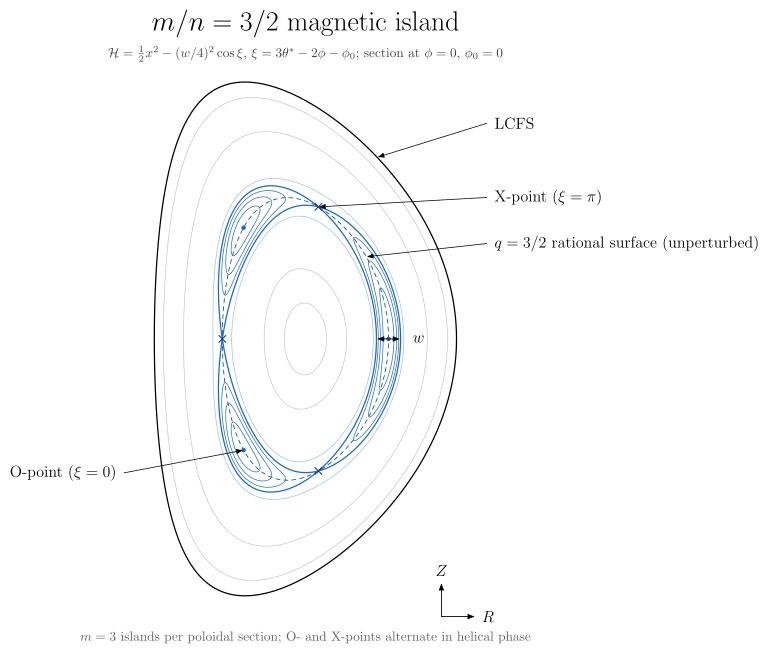
vaft.diagram.magnetic_island(m=3, n=2, width=0.16, phase=0.0, r_s=0.55, elongation=1.7, triangularity=0.4, projection='poloidal')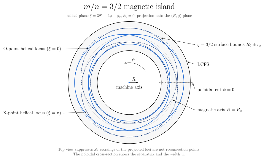
vaft.diagram.magnetic_island(m=3, n=2, width=0.16, phase=0.0, r_s=0.55, elongation=1.7, triangularity=0.4, projection='top')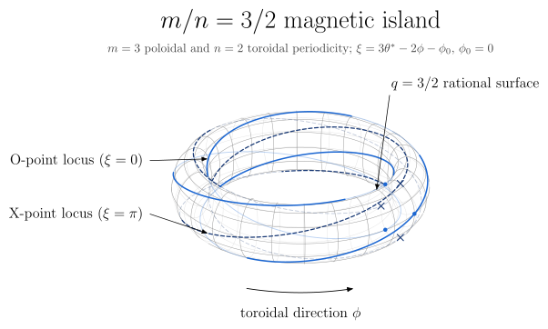
vaft.diagram.magnetic_island(m=3, n=2, width=0.16, phase=0.0, r_s=0.55, elongation=1.7, triangularity=0.4, projection='3d')Schematic of an $m/n$ magnetic island in one of three projections.
vaft.diagram.magnetic_island(m=2, n=1, width=0.24, phase=0.0, projection='poloidal', *, r_s=0.64, aspect_ratio=3.2, elongation=1.0, triangularity=0.0, show_rational_surface=True, show_separatrix=True, show_o_points=True, show_x_points=True, labels=True, time=None, rotation_frequency=None, animation=False, fps=None, duration=None, dpi=None, frame_label=None)Formats .svg .tex .pdf the SVG above is committed; build the others locally
import vaft.diagram

d = vaft.diagram.magnetic_island(m=3, n=2, width=0.16, phase=0.0, r_s=0.55, elongation=1.7, triangularity=0.4, projection='poloidal')
d.tikz  # the TikZ document as text
d.save("magnetic_island_poloidal.svg")  # rendered vector image, the canonical artifact; needs latex, dvisvgm
d.save("magnetic_island_poloidal.tex")  # the complete TikZ document, the text source
d.save("magnetic_island_poloidal.pdf")  # vector PDF; needs pdflatex
Formula functions referenced:
equilibrium.miller_surface, equilibrium.straight_field_line_angle, stability.helical_phase, stability.island_pendulum_hamiltonian, stability.island_separatrix_half_width
Stability and operational-space diagrams: textbook 2-D projections
Module vaft.diagram._stability_space
peeling_ballooning
1 asset
source
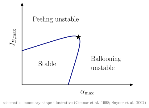
vaft.diagram.peeling_ballooning()Schematic edge-stability (peeling-ballooning) diagram.
vaft.diagram.peeling_ballooning(*, labels=True)Show source vaft/diagram/_stability_space.py, lines 107–133
def peeling_ballooning(*, labels: bool = True) -> Diagram:
    r"""Schematic edge-stability (peeling-ballooning) diagram.

    Axes are the pedestal's peak normalised pressure gradient
    $\alpha_\mathrm{max}$ and peak bootstrap (edge) current density
    $J_{B,\mathrm{max}}$, in arbitrary units: the boundary's shape is
    illustrative, not computed from an equilibrium. Its corner, where the
    peeling and ballooning limits meet (the star), is where ELM-limited
    pedestals typically sit; it is computed from the model, not placed.
    """
    model = PeelingBallooningModel()
    chart = Chart(x_range=(0.0, 1.25), y_range=(0.0, 1.0))
    chart.curves["boundary"] = model.boundary()
    chart.points["corner"] = model.corner()
    chart.labels.update({"peeling": (0.4, 0.86), "stable": (0.3, 0.28), "ballooning": (1.0, 0.28)})
    chart.parameters.update({k: getattr(model, k) for k in ("j0", "j_slope", "a0", "a_slope", "width", "tau")})
    scene = _render_chart(
        chart,
        x_label="$\\alpha_\\mathrm{max}$",
        y_label="$J_{B,\\mathrm{max}}$",
        curve_styles={"boundary": "boundary"},
        region_text={"peeling": "Peeling unstable", "stable": "Stable",
                     "ballooning": "\\begin{tabular}{l}Ballooning\\\\unstable\\end{tabular}"} if labels else {},
        note="schematic: boundary shape illustrative (Connor et al. 1998; Snyder et al. 2002)" if labels else "",
        star="corner",
    )
    return Diagram("peeling_ballooning", scene, model=chart)
Formats .svg .tex .pdf the SVG above is committed; build the others locally
import vaft.diagram

d = vaft.diagram.peeling_ballooning()
d.tikz  # the TikZ document as text
d.save("peeling_ballooning.svg")  # rendered vector image, the canonical artifact; needs latex, dvisvgm
d.save("peeling_ballooning.tex")  # the complete TikZ document, the text source
d.save("peeling_ballooning.pdf")  # vector PDF; needs pdflatex
s_alpha_ballooning
1 asset
source
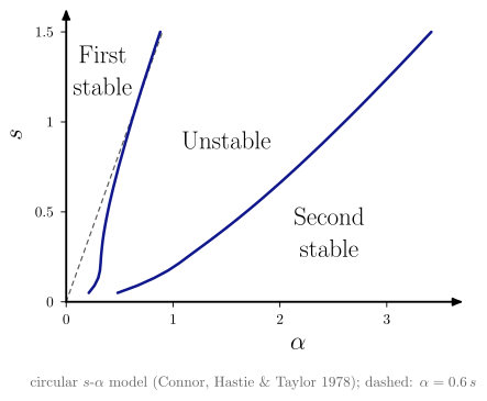
vaft.diagram.s_alpha_ballooning()First and second ballooning stability in the circular $s$-$\alpha$ model.
vaft.diagram.s_alpha_ballooning(*, s_max=1.5, alpha_max=3.5, labels=True)Show source vaft/diagram/_stability_space.py, lines 148–191
def s_alpha_ballooning(*, s_max: float = 1.5, alpha_max: float = 3.5, labels: bool = True) -> Diagram:
    r"""First and second ballooning stability in the circular $s$-$\alpha$ model.

    Both boundaries come from ``vaft.formula.s_alpha_marginal_alpha``; the
    dashed line is the $\alpha = 0.6\,s$ approximation
    ``ballooning_stability_criterion`` uses.
    """
    if not 0.1 < s_max <= 2.5 or not 0.5 < alpha_max <= 6.0:
        raise ValueError("s_max must lie in (0.1, 2.5] and alpha_max in (0.5, 6]")
    s, first, second = _s_alpha_boundaries(0.05, float(s_max), 36)
    ok = np.isfinite(first)
    chart = Chart(x_range=(0.0, float(alpha_max)), y_range=(0.0, float(s_max)))
    # two open branches: below s ~ 0.05 the model's boundaries are not resolved
    chart.curves["first"] = np.stack([first[ok], s[ok]], axis=-1)
    second_ok = ok & np.isfinite(second)
    chart.curves["second"] = np.stack([second[second_ok], s[second_ok]], axis=-1)
    chart.curves["approximation"] = np.array([[0.0, 0.0], [0.6 * s_max, s_max]])
    # labels are placed from the computed boundaries, so they stay in their
    # regions whatever the axis ranges; a region off the chart gets none
    def at(row, curve):
        return float(np.interp(row, s[ok], curve[ok]))

    s_first, s_unstable, s_second = 0.85 * s_max, 0.6 * s_max, max(0.25 * s_max, 0.1)
    a1 = at(s_first, first)
    chart.labels["first"] = (0.45 * a1, s_first)
    a1, a2 = at(s_unstable, first), at(s_unstable, np.where(np.isfinite(second), second, alpha_max))
    if a1 < 0.9 * alpha_max:
        chart.labels["unstable"] = (0.5 * (a1 + min(a2, alpha_max)), s_unstable)
    a2 = at(s_second, np.where(np.isfinite(second), second, np.inf))
    if a2 < 0.75 * alpha_max:
        chart.labels["second"] = (0.5 * (a2 + alpha_max), s_second)
    chart.parameters.update({"s_min": 0.05, "s_max": float(s_max), "alpha_max": float(alpha_max)})
    scene = _render_chart(
        chart,
        x_label="$\\alpha$",
        y_label="$s$",
        curve_styles={"approximation": "approx", "first": "boundary", "second": "boundary"},
        region_text={k: v for k, v in {
            "first": "\\begin{tabular}{c}First\\\\stable\\end{tabular}", "unstable": "Unstable",
            "second": "\\begin{tabular}{c}Second\\\\stable\\end{tabular}"}.items() if k in chart.labels} if labels else {},
        x_ticks=_nice_ticks(alpha_max + 1e-9), y_ticks=_nice_ticks(s_max + 1e-9),
        note="circular $s$-$\\alpha$ model (Connor, Hastie \\& Taylor 1978); dashed: $\\alpha = 0.6\\,s$" if labels else "",
    )
    return Diagram("s_alpha_ballooning", scene, model=chart)
Formats .svg .tex .pdf the SVG above is committed; build the others locally
import vaft.diagram

d = vaft.diagram.s_alpha_ballooning()
d.tikz  # the TikZ document as text
d.save("s_alpha_ballooning.svg")  # rendered vector image, the canonical artifact; needs latex, dvisvgm
d.save("s_alpha_ballooning.tex")  # the complete TikZ document, the text source
d.save("s_alpha_ballooning.pdf")  # vector PDF; needs pdflatex
Formula functions referenced:
stability.s_alpha_marginal_alpha
hugill
1 asset
source
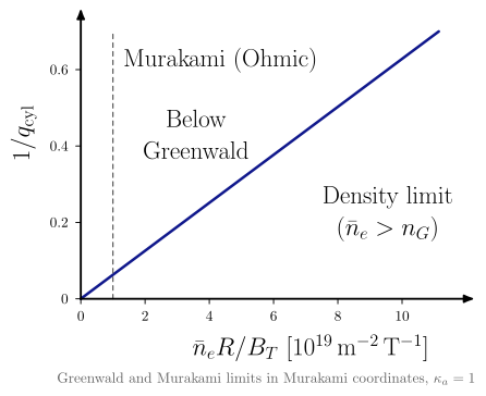
vaft.diagram.hugill()Hugill diagram: $1/q_\mathrm{cyl}$ against the Murakami parameter $\bar n R/B$.
vaft.diagram.hugill(*, elongation=1.0, q_limit=None, labels=True)Show source vaft/diagram/_stability_space.py, lines 228–284
def hugill(*, elongation: float = 1.0, q_limit: Optional[float] = None, labels: bool = True) -> Diagram:
    r"""Hugill diagram: $1/q_\mathrm{cyl}$ against the Murakami parameter $\bar n R/B$.

    The lines are the registered boundaries of the ``hugill`` projection
    (:mod:`vaft.formula.boundaries`, #1425): ``greenwald_hugill``, the
    Greenwald density in these coordinates, a straight line through the
    origin $1/q_\mathrm{cyl} = (\pi/50\kappa_a)\,\bar nR/B$ ($\bar n$ in
    $10^{19}\,\mathrm{m^{-3}}$) whose slope depends only on the area
    elongation; and ``murakami_hugill``, the vertical line $\bar nR/B = 1$.

    The registered current limit ``low_q`` is $q_\psi > 2$, the equilibrium
    edge q, not the $q_\mathrm{cyl}$ on this axis, so it is not drawn. Passing
    ``q_limit`` adds a horizontal *reference* line $q_\mathrm{cyl} = q_\mathrm{limit}$,
    labelled as such; it is not a registered boundary.
    """
    _validate_shape(_HUGILL_ASPECT_RATIO, elongation, q_limit)
    q_size = q_limit if q_limit is not None else _SIZING_Q
    y_max = 1.4 / q_size
    x_q = float(_b.boundary_value(_b.get_boundary("greenwald_hugill"),
                                  inverse_cylindrical_q=1.0 / q_size, area_elongation=elongation))
    x_max = 1.45 * x_q
    plan = overlay_plan("hugill", x_range=(0.0, x_max), y_range=(0.0, y_max),
                        fixed={"area_elongation": elongation})
    curves = {c.key: c for c in plan.curves}
    chart = Chart(x_range=(0.0, x_max), y_range=(0.0, y_max))
    chart.curves["greenwald"] = curves["greenwald_hugill"].xy
    chart.curves["murakami"] = curves["murakami_hugill"].xy
    # Murakami is a soft, Ohmic-era scaling: dashed, so the solid line stays the Greenwald limit
    styles = {"greenwald": "boundary", "murakami": "approx"}
    x_m = float(_b.boundary_value(_b.get_boundary("murakami_hugill")))
    chart.labels.update({
        "accessible": (0.45 * x_q, 0.85 / q_size),
        "density": (1.2 * x_q, 0.45 / q_size),
        "murakami": (x_m + 0.42 * x_q, 1.25 / q_size),
    })
    text = {"accessible": "\\begin{tabular}{c}Below\\\\Greenwald\\end{tabular}",
            "density": "\\begin{tabular}{c}Density limit\\\\($\\bar n_e > n_G$)\\end{tabular}",
            "murakami": "Murakami (Ohmic)"}
    if q_limit is not None:
        chart.curves["low_q"] = np.array([[0.0, 1.0 / q_limit], [x_max, 1.0 / q_limit]])
        styles["low_q"] = "approx"
        chart.labels["low_q"] = (0.33 * x_max, 1.2 / q_limit)
        text["low_q"] = f"Reference $q_\\mathrm{{cyl}} = {q_limit:g}$ (not $q_\\psi$)"
    chart.parameters.update({"elongation": elongation, "q_limit": q_limit, "murakami_at_q_limit": x_q,
                             "boundaries": plan.keys})
    scene = _render_chart(
        chart,
        x_label="$\\bar n_e R/B_T\\ [10^{19}\\,\\mathrm{m^{-2}\\,T^{-1}}]$",
        y_label="$1/q_\\mathrm{cyl}$",
        curve_styles=styles,
        region_text=text if labels else {},
        x_ticks=_nice_ticks(x_max),
        y_ticks=_nice_ticks(y_max),
        note=(f"Greenwald and Murakami limits in Murakami coordinates, $\\kappa_a = {elongation:g}$"
              if labels else ""),
    )
    return Diagram("hugill", scene, model=chart)
Formats .svg .tex .pdf the SVG above is committed; build the others locally
import vaft.diagram

d = vaft.diagram.hugill()
d.tikz  # the TikZ document as text
d.save("hugill.svg")  # rendered vector image, the canonical artifact; needs latex, dvisvgm
d.save("hugill.tex")  # the complete TikZ document, the text source
d.save("hugill.pdf")  # vector PDF; needs pdflatex
hugill_st
1 asset
source
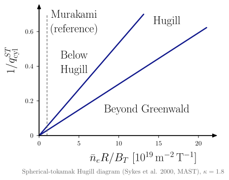
vaft.diagram.hugill_st()Spherical-tokamak Hugill diagram: $1/q^{ST}_\mathrm{cyl}$ against $\bar n R/B$ (Sykes et al. 2000, MAST).
vaft.diagram.hugill_st(*, elongation=1.8, labels=True)Show source vaft/diagram/_stability_space.py, lines 287–338
def hugill_st(*, elongation: float = 1.8, labels: bool = True) -> Diagram:
    r"""Spherical-tokamak Hugill diagram: $1/q^{ST}_\mathrm{cyl}$ against $\bar n R/B$ (Sykes et al. 2000, MAST).

    The vertical coordinate is the spherical-tokamak cylindrical safety factor
    $q^{ST}_\mathrm{cyl} = 2.5\,a^2(1+\kappa^2)B_T/(R I_p)$ of Sykes et al. (MAST,
    IAEA FEC 2000, Fig. 12), not the conventional $q_\mathrm{cyl}$ of
    :func:`hugill`. The lines are the registered boundaries of the
    ``hugill_st`` projection: ``sykes_2000_st_hugill``, the Hugill limit as
    Sykes et al. define it ($n_H = I_p/\pi a^2\kappa$), and
    ``greenwald_hugill_st``, the unchanged Greenwald limit on these axes, both
    lines through the origin whose slopes depend on $\kappa$ (MAST's figure
    uses 1.8); and ``murakami_hugill``, drawn dashed as a historical
    conventional-tokamak reference only.
    """
    _validate_shape(_HUGILL_ASPECT_RATIO, elongation, None)
    y_max = 1.4 / _SIZING_Q
    x_q = float(_b.boundary_value(_b.get_boundary("greenwald_hugill_st"),
                                  inverse_cylindrical_q_st=1.0 / _SIZING_Q, elongation=elongation))
    x_max = 1.25 * x_q
    plan = overlay_plan("hugill_st", x_range=(0.0, x_max), y_range=(0.0, y_max), fixed={"elongation": elongation})
    curves = {c.key: c for c in plan.curves}
    chart = Chart(x_range=(0.0, x_max), y_range=(0.0, y_max))
    chart.curves["greenwald"] = curves["greenwald_hugill_st"].xy
    chart.curves["hugill"] = curves["sykes_2000_st_hugill"].xy
    chart.curves["murakami"] = curves["murakami_hugill"].xy
    styles = {"greenwald": "boundary", "hugill": "boundary", "murakami": "approx"}
    x_m = float(_b.boundary_value(_b.get_boundary("murakami_hugill")))
    # each label in its own zone, clear of the three lines: below Hugill between Murakami and the Hugill line,
    # the Hugill name between the Hugill and Greenwald lines, Greenwald beyond its line, Murakami right of x = 1
    chart.labels.update({
        "accessible": (0.26 * x_q, 0.84 / _SIZING_Q),
        "hugill": (0.95 * x_q, 1.32 / _SIZING_Q),   # past the top end of the Hugill line, left of Greenwald
        "density": (0.80 * x_q, 0.30 / _SIZING_Q),
        "murakami": (x_m + 0.20 * x_q, 1.31 / _SIZING_Q),
    })
    text = {"accessible": "\\begin{tabular}{c}Below\\\\Hugill\\end{tabular}",
            "hugill": "Hugill",
            "density": "Beyond Greenwald",
            "murakami": "\\begin{tabular}{c}Murakami\\\\(reference)\\end{tabular}"}
    chart.parameters.update({"elongation": elongation, "boundaries": plan.keys})
    scene = _render_chart(
        chart,
        x_label="$\\bar n_e R/B_T\\ [10^{19}\\,\\mathrm{m^{-2}\\,T^{-1}}]$",
        y_label="$1/q^{ST}_\\mathrm{cyl}$",
        curve_styles=styles,
        region_text=text if labels else {},
        x_ticks=_nice_ticks(x_max),
        y_ticks=_nice_ticks(y_max),
        note=(f"Spherical-tokamak Hugill diagram (Sykes et al. 2000, MAST), $\\kappa = {elongation:g}$"
              if labels else ""),
    )
    return Diagram("hugill_st", scene, model=chart)
Formats .svg .tex .pdf the SVG above is committed; build the others locally
import vaft.diagram

d = vaft.diagram.hugill_st()
d.tikz  # the TikZ document as text
d.save("hugill_st.svg")  # rendered vector image, the canonical artifact; needs latex, dvisvgm
d.save("hugill_st.tex")  # the complete TikZ document, the text source
d.save("hugill_st.pdf")  # vector PDF; needs pdflatex
troyon
1 asset
source
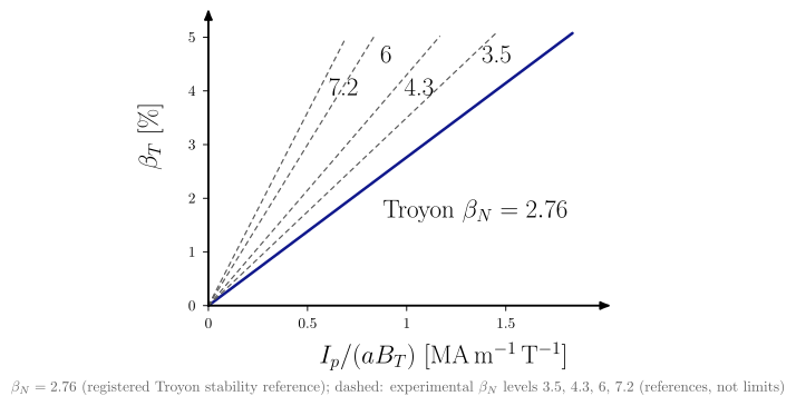
vaft.diagram.troyon()Troyon diagram: toroidal beta against the normalised current $I_p/(aB_T)$.
vaft.diagram.troyon(*, beta_N_max=None, aspect_ratio=3.0, elongation=1.7, q_limit=None, labels=True)Show source vaft/diagram/_stability_space.py, lines 341–414
def troyon(*, beta_N_max: Optional[float] = None, aspect_ratio: float = 3.0, elongation: float = 1.7,
           q_limit: Optional[float] = None, labels: bool = True) -> Diagram:
    r"""Troyon diagram: toroidal beta against the normalised current $I_p/(aB_T)$.

    The registered ``troyon`` stability reference
    ($\beta_N = 2.2\,\mu_0 \cdot 10^6 \approx 2.76$, :mod:`vaft.formula.boundaries`) is
    drawn through the definition of $\beta_N$, $\beta_T[\%] = \beta_N\,I_p/(aB_T)$,
    with the projection's experimental references (#1691: DIII-D, ST, NSTX levels)
    dashed beside it. None is a limit, so no side is marked stable or unstable.
    ``beta_N_max`` overrides the Troyon value for a what-if picture, and the note
    then says so.

    No current limit is drawn by default: the registered ``low_q`` is on
    $q_\psi$, and this axis is $q_\mathrm{cyl}$-like. ``q_limit`` adds a
    *reference* cutoff where ``q_cyl_from_B_R_epsilon_kappa_I`` reaches it,
    at $I_p/(aB_T) = 5\varepsilon\kappa_a/q_\mathrm{limit}$.
    """
    _validate_shape(aspect_ratio, elongation, q_limit)
    if beta_N_max is not None and not beta_N_max > 0.0:
        raise ValueError(f"beta_N_max must be positive, not {beta_N_max!r}")
    registered = float(_b.boundary_value(_b.get_boundary("troyon")))
    level = registered if beta_N_max is None else float(beta_N_max)
    a = _R0 / aspect_ratio
    x_q = _current_at_q(elongation, aspect_ratio, q_limit if q_limit is not None else _SIZING_Q) / (a * _B0)
    x_max = 1.35 * x_q
    y_max = 1.3 * level * x_q
    chart = Chart(x_range=(0.0, float(x_max)), y_range=(0.0, float(y_max)))
    plan = overlay_plan("troyon", x_range=(0.0, x_max), y_range=(0.0, y_max), samples=101)
    if beta_N_max is None:
        chart.curves["beta_limit"] = next(c for c in plan.curves if c.key == "troyon").xy
    else:
        x = np.linspace(0.0, x_max, 101)
        chart.curves["beta_limit"] = np.stack([x, level * x], axis=-1)
    styles = {"beta_limit": "boundary"}
    # the Troyon name below its line, the experimental references' names where each meets the top of the frame
    chart.labels["beta"] = (0.95 * x_q, 0.45 * level * x_q)
    text = {"beta": f"Troyon $\\beta_N = {level:.3g}$"}
    for k, curve in enumerate(c for c in plan.curves if c.key != "troyon"):
        entry = _b.get_boundary(curve.key)
        name = f"ref{k}"
        chart.curves[name] = curve.xy
        styles[name] = "approx"
        # just right of its line, alternating heights so neighbouring steep lines keep their names apart
        y_label = (0.92 - 0.12 * (k % 2)) * y_max
        x_label = y_label / float(entry.coefficient) + 0.06 * x_max
        if x_label < 0.97 * x_max:
            chart.labels[name] = (x_label, y_label)
            text[name] = f"{entry.coefficient:.3g}"
    if q_limit is not None:
        chart.curves["low_q"] = np.array([[x_q, 0.0], [x_q, y_max]])
        styles["low_q"] = "approx"
        chart.labels["low_q"] = (1.18 * x_q, 0.45 * level * x_q)
        text["low_q"] = "\\begin{tabular}{c}Reference\\\\$q_\\mathrm{cyl}$\\end{tabular}"
    chart.parameters.update({"beta_N_max": level, "beta_N_registered": registered, "aspect_ratio": aspect_ratio,
                             "elongation": elongation, "q_limit": q_limit, "current_at_q_limit": x_q})
    source = "registered Troyon stability reference" if beta_N_max is None else "user value, not the registered one"
    levels = ", ".join(f"{_b.get_boundary(c.key).coefficient:.3g}" for c in plan.curves if c.key != "troyon")
    note = f"$\\beta_N = {level:.3g}$ ({source})"
    if levels:   # the values from the registry, never restated here
        note += f"; dashed: experimental $\\beta_N$ levels {levels} (references, not limits)"
    if q_limit is not None:
        note += (f"; $q_\\mathrm{{cyl}} = {q_limit:g}$ at $R_0/a = {aspect_ratio:g}$, "
                 f"$\\kappa_a = {elongation:g}$")
    scene = _render_chart(
        chart,
        x_label="$I_p/(aB_T)\\ [\\mathrm{MA\\,m^{-1}\\,T^{-1}}]$",
        y_label="$\\beta_T\\ [\\%]$",
        curve_styles=styles,
        region_text=text if labels else {},
        x_ticks=_nice_ticks(float(x_max)),
        y_ticks=_nice_ticks(float(y_max)),
        note=note if labels else "",
    )
    return Diagram("troyon", scene, model=chart)
Formats .svg .tex .pdf the SVG above is committed; build the others locally
import vaft.diagram

d = vaft.diagram.troyon()
d.tikz  # the TikZ document as text
d.save("troyon.svg")  # rendered vector image, the canonical artifact; needs latex, dvisvgm
d.save("troyon.tex")  # the complete TikZ document, the text source
d.save("troyon.pdf")  # vector PDF; needs pdflatex
Formula functions referenced:
equilibrium.q_cyl_from_B_R_epsilon_kappa_I
Equilibrium-derived analytic and reduced MHD stability diagnostics
Module vaft.diagram._reduced_stability
stability_diagnostic_taxonomy
1 asset
source
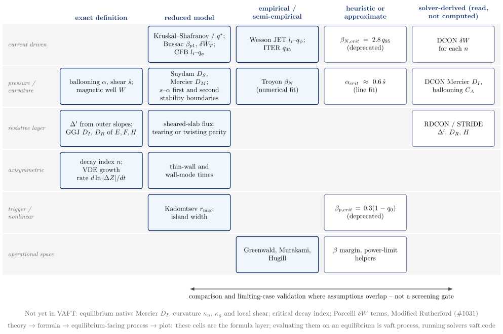
vaft.diagram.stability_diagnostic_taxonomy()Reduced MHD stability diagnostics by physical problem and logical status.
vaft.diagram.stability_diagnostic_taxonomy(*, labels=True)Show source vaft/diagram/_reduced_stability.py, lines 94–150
def stability_diagnostic_taxonomy(*, labels: bool = True) -> Diagram:
    r"""Reduced MHD stability diagnostics by physical problem and logical status.

    Rows are the physical problem (current driven, pressure / curvature,
    resistive layer, axisymmetric, trigger / nonlinear, operational space),
    columns the logical status: exact definition, reduced model, empirical
    or semi-empirical boundary, heuristic or approximate, and solver-derived
    (DCON / RDCON / STRIDE quantities VAFT reads but does not compute). Each
    cell names what ``vaft.formula`` holds there; the gaps are listed. The
    reduced columns are compared with the solver column -- interpretation
    and limiting-case validation, not a screening gate.
    """
    labels = _check_labels(labels)
    items: List = []
    width = len(STATUSES) * (_CELL_W + 0.3)
    left = _X0 - 0.5 * _CELL_W - 3.0
    right = _X0 - 0.5 * _CELL_W + width
    for j, (key, text) in enumerate(STATUSES):
        x, _ = _cell_center(0, j)
        items.append(Label((x, _Y0 + 0.5 * _CELL_H + 0.2), text, "concept group title,text width=4.1cm,align=center",
                           anchor="south", role=f"status:{key}"))
    for i, (key, text) in enumerate(PROBLEMS):
        _, y = _cell_center(i, 0)
        items += band(left, right, y - 0.5 * _CELL_H - 0.12, y + 0.5 * _CELL_H + 0.12, role=f"problem:{key}")
        items.append(Label((left + 0.15, y), text, "concept band label,text width=2.6cm,align=left,execute at begin node={\\hyphenpenalty=10000}", anchor="west",
                           role=f"problem:{key}"))
    cells = {}
    for i, (problem, _) in enumerate(PROBLEMS):
        for j, (status, _) in enumerate(STATUSES):
            text = CELLS.get((problem, status))
            if text is None:
                continue
            x, y = _cell_center(i, j)
            style = "concept leaf" if status in ("heuristic", "solver") else "concept box"
            cells[(problem, status)] = box(x, y, _CELL_W, _CELL_H, text, style=style,
                                           role=f"cell:{problem}:{status}", latex=True)
            items += list(cells[(problem, status)].items)
    bottom = _cell_center(len(PROBLEMS) - 1, 0)[1] - 0.5 * _CELL_H - 0.4
    # the reduced and definition columns are compared with the solver column, not gated by it
    y_cmp = bottom - 0.45
    x_from = _cell_center(0, 1)[0]
    x_to = _cell_center(0, 4)[0]
    items.append(Arrow((x_from, y_cmp), (x_to, y_cmp), "connector both", role="comparison"))
    items.append(Label((0.5 * (x_from + x_to), y_cmp - 0.12),
                       "comparison and limiting-case validation where assumptions overlap -- not a screening gate",
                       "small label", anchor="north", role="comparison"))
    if labels:
        items.append(Label((0.5 * (left + right), y_cmp - 1.0),
                           "Not yet in VAFT: " + "; ".join(ABSENT), "note", anchor="north", role="note"))
        items.append(Label((0.5 * (left + right), y_cmp - 1.65),
                           "theory $\\to$ formula $\\to$ equilibrium-facing process $\\to$ plot: these cells are the "
                           "formula layer; evaluating them on an equilibrium is vaft.process, running solvers vaft.code",
                           "note", anchor="north", role="note"))
    model = {"statuses": tuple(k for k, _ in STATUSES), "problems": tuple(k for k, _ in PROBLEMS),
             "cells": dict(CELLS), "absent": ABSENT,
             "centers": {k: (b.x, b.y) for k, b in cells.items()}}
    return Diagram("stability_diagnostic_taxonomy", Scene(tuple(items)), model=model)
Formats .svg .tex .pdf the SVG above is committed; build the others locally
import vaft.diagram

d = vaft.diagram.stability_diagnostic_taxonomy()
d.tikz  # the TikZ document as text
d.save("stability_diagnostic_taxonomy.svg")  # rendered vector image, the canonical artifact; needs latex, dvisvgm
d.save("stability_diagnostic_taxonomy.tex")  # the complete TikZ document, the text source
d.save("stability_diagnostic_taxonomy.pdf")  # vector PDF; needs pdflatex
interchange_criteria
1 asset
source
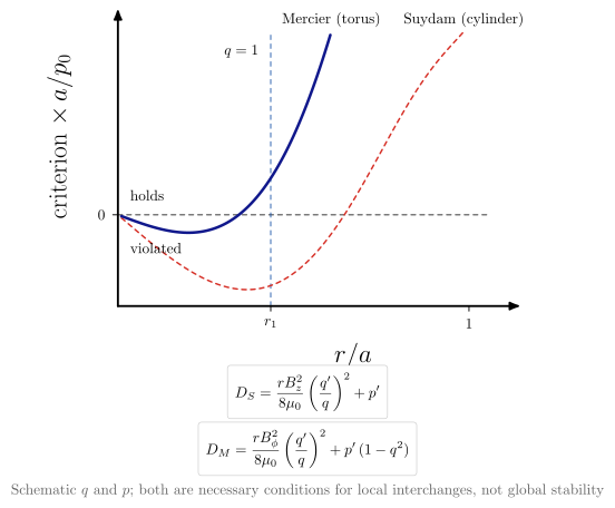
vaft.diagram.interchange_criteria()Suydam’s and Mercier’s local interchange criteria across one schematic profile.
vaft.diagram.interchange_criteria(*, labels=True)Show source vaft/diagram/_reduced_stability.py, lines 161–223
def interchange_criteria(*, labels: bool = True) -> Diagram:
    r"""Suydam's and Mercier's local interchange criteria across one schematic profile.

    $q(r)$ is Wesson's peaked-current profile (``peaked_current_safety_factor``,
    $q_a = 3$, $\nu = 3$, so $q_0 = 0.75$) and $p \propto (1 - r^2/a^2)^2$. Both
    criteria (``suydam_criterion``, ``mercier_criterion_circular``) are
    normalised by $p_0/a$; positive means the criterion holds. Mercier is
    Suydam plus $-p'q^2$: outward pressure fall stabilises outside $q = 1$,
    so its violated region stays inside $r_1$ while Suydam's extends past it.
    Both are necessary conditions for local interchanges, not global
    stability.
    """
    labels = _check_labels(labels)
    x = np.linspace(0.01, 1.0, 397)
    r = _A * x
    q = peaked_current_safety_factor(x, _Q_A, _NU)
    p = _P0 * (1.0 - x ** 2) ** 2
    dq, dp = gradient(r, q), gradient(r, p)
    scale = _A / _P0
    suydam = suydam_criterion(r, _B, q, dq, dp) * scale
    mercier = mercier_criterion_circular(r, _B, q, dq, dp) * scale
    r1 = float(np.interp(1.0, q, x))
    lo, hi = -1.2, 2.4
    chart = Chart(x_range=(0.0, 1.08), y_range=(lo, hi))
    chart.curves.update({
        "suydam": np.stack([x, suydam], -1), "mercier": np.stack([x, mercier], -1),
        "zero": np.array([[0.0, 0.0], [1.05, 0.0]]), "q_one": np.array([[r1, lo], [r1, hi]]),
    })

    def exit_x(values):
        return float(x[np.argmax(values >= hi)])

    def last_violation(values):
        return float(x[values < 0.0].max()) if np.any(values < 0.0) else 0.0

    chart.parameters.update({"q_a": _Q_A, "nu": _NU, "q0": float(q[0]), "r1": r1,
                             "suydam_violated_to": last_violation(suydam),
                             "mercier_violated_to": last_violation(mercier)})
    scene = render_chart(chart, x_label="$r/a$", y_label="criterion $\\times\\, a/p_0$", y_ticks=(0.0,),
                         curve_styles={"zero": "approx", "q_one": "rational", "suydam": "slope plus",
                                       "mercier": "outer solution"},
                         region_text={}, x_ticks=(r1, 1.0), x_tick_text=("$r_1$", "$1$"))
    items: List = []
    if labels:
        at = chart.to_cm
        items += [
            # each curve is named where it leaves the top of the frame
            Label(tuple(at(np.array([exit_x(mercier), hi]))), "Mercier (torus)", "small label",
                  anchor="south", role="mercier"),
            Label(tuple(at(np.array([exit_x(suydam), hi]))), "Suydam (cylinder)", "small label",
                  anchor="south", role="suydam"),
            Label(tuple(at(np.array([r1 - 0.02, hi - 0.1]))), "$q = 1$", "small label", anchor="north east",
                  role="q_one"),
            Label(tuple(at(np.array([0.02, 0.12]))), "holds", "small label", anchor="south west", role="sign"),
            Label(tuple(at(np.array([0.02, -0.3]))), "violated", "small label", anchor="north west", role="sign"),
            Label((CHART_WIDTH / 2, -1.4), f"$\\displaystyle {formula_equation(suydam_criterion)}$", "formula box",
                  anchor="north", role="equations"),
            Label((CHART_WIDTH / 2, -2.75), f"$\\displaystyle {formula_equation(mercier_criterion_circular)}$",
                  "formula box", anchor="north", role="equations"),
            Label((CHART_WIDTH / 2, -4.1), "Schematic $q$ and $p$; both are necessary conditions for local "
                  "interchanges, not global stability", "note", anchor="north", role="note"),
        ]
    return Diagram("interchange_criteria", scene + Scene(tuple(items)), model=chart)
Formats .svg .tex .pdf the SVG above is committed; build the others locally
import vaft.diagram

d = vaft.diagram.interchange_criteria()
d.tikz  # the TikZ document as text
d.save("interchange_criteria.svg")  # rendered vector image, the canonical artifact; needs latex, dvisvgm
d.save("interchange_criteria.tex")  # the complete TikZ document, the text source
d.save("interchange_criteria.pdf")  # vector PDF; needs pdflatex
Formula functions referenced:
geometry.peaked_current_safety_factor, stability.mercier_criterion_circular, stability.suydam_criterion, utils.gradient
Reduced and full-geometry high-$n$ ballooning formulations side by side
Module vaft.diagram._ballooning_formulations
ballooning_formulation_hierarchy
1 asset
source
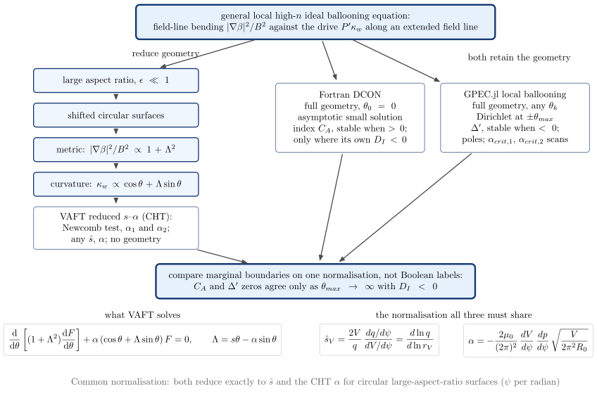
vaft.diagram.ballooning_formulation_hierarchy()How the reduced $s$-$\alpha$ model and the full-geometry ballooning codes relate.
vaft.diagram.ballooning_formulation_hierarchy(*, labels=True)Show source vaft/diagram/_ballooning_formulations.py, lines 47–125
def ballooning_formulation_hierarchy(*, labels: bool = True) -> Diagram:
    r"""How the reduced $s$-$\alpha$ model and the full-geometry ballooning codes relate.

    The general local high-$n$ ideal ballooning equation (field-line bending
    against the pressure-curvature drive) either loses its geometry step by
    step -- large aspect ratio, shifted circles, the $1 + \Lambda^2$ metric,
    the $\cos\theta + \Lambda\sin\theta$ curvature -- to become the
    Connor-Hastie-Taylor equation of ``s_alpha_ballooning_stable``, or keeps
    it, as Fortran DCON (asymptotic matching, $C_A$, stable when positive)
    and GPEC.jl (Dirichlet matching, ballooning $\Delta'$, stable when
    negative, with poles) do. Their marginal boundaries are comparable only
    after a common normalisation: ``shear_from_volume`` and
    ``ballooning_alpha_from_volume``, which reduce exactly to $\hat s$ and the
    CHT $\alpha$ for circles.
    """
    labels = _check_labels(labels)
    items: List = []
    nodes = {
        "general": box(2.9, 0.0, 13.5, 1.3, "general local high-$n$ ideal ballooning equation:\\\\ field-line bending "
                       "$|\\nabla\\beta|^2/B^2$ against the drive $P'\\kappa_w$ along an extended field line",
                       style="concept strong", role="node:general", latex=True),
    }
    y = -2.2
    for key, text in REDUCTION_STEPS:
        nodes[key] = box(_X_LEFT, y, 6.2, 0.9, text, role=f"node:{key}", latex=True)
        y -= 1.3
    nodes["vaft"] = box(_X_LEFT, y - 0.35, 6.2, 1.6, "VAFT reduced $s$--$\\alpha$ (CHT):\\\\ Newcomb test, "
                        "$\\alpha_1$ and $\\alpha_2$;\\\\ any $\\hat s$, $\\alpha$; no geometry", style="concept leaf",
                        role="node:vaft", latex=True)
    nodes["dcon"] = box(_X_DCON, -3.6, 5.6, 2.6, "Fortran DCON\\\\ full geometry, $\\theta_0 = 0$\\\\ asymptotic "
                        "small solution\\\\ index $C_A$, stable when $> 0$;\\\\ only where its own $D_I < 0$",
                        style="concept leaf", role="node:dcon", latex=True)
    nodes["gpec_jl"] = box(_X_JL, -3.6, 5.6, 2.6, "GPEC.jl local ballooning\\\\ full geometry, any $\\theta_k$\\\\ "
                           "Dirichlet at $\\pm\\theta_{max}$\\\\ $\\Delta'$, stable when $< 0$;\\\\ poles; "
                           "$\\alpha_{crit,1}$, $\\alpha_{crit,2}$ scans", style="concept leaf",
                           role="node:gpec_jl", latex=True)
    compare_y = nodes["vaft"].y - 2.0
    nodes["compare"] = box(2.9, compare_y, 12.0, 1.3, "compare marginal boundaries on one normalisation, not Boolean labels:\\\\ "
                           "$C_A$ and $\\Delta'$ zeros agree only as $\\theta_{max} \\to \\infty$ with $D_I < 0$", style="concept strong", role="node:compare",
                           latex=True)
    for b in nodes.values():
        items += list(b.items)
    edges = [("general", "large_aspect_ratio", "reduce geometry"), ("large_aspect_ratio", "shifted_circles", ""),
             ("shifted_circles", "metric", ""), ("metric", "curvature", ""), ("curvature", "vaft", ""),
             ("general", "dcon", ""), ("general", "gpec_jl", ""),
             ("vaft", "compare", ""), ("dcon", "compare", ""), ("gpec_jl", "compare", "")]
    for a, b, text in edges:
        arrow = connector(nodes[a], nodes[b], role=f"edge:{a}->{b}")
        items.append(arrow)
        if text and labels:
            mx, my = 0.5 * (arrow.start[0] + arrow.end[0]), 0.5 * (arrow.start[1] + arrow.end[1])
            side = "east" if mx < nodes["general"].x - 2.0 else "west"
            items.append(Label((mx + (-0.15 if side == "east" else 0.15), my), text, "small label", anchor=side,
                               role=f"edge:{a}->{b}"))
    if labels:
        # one label for both full-geometry arrows, right of the GPEC.jl one
        items.append(Label((8.5, -1.35), "both retain the geometry", "small label", anchor="west",
                           role="edge:general->full"))
    # the equations: what VAFT solves, and the normalisation all three must share
    eq_y = compare_y - 1.6
    items += [
        Label((-3.6, eq_y), f"$\\displaystyle {formula_equation(s_alpha_ballooning_stable)}$",
              "formula box", anchor="north", role="equation:cht"),
        Label((5.3, eq_y), f"$\\displaystyle {formula_equation(shear_from_volume)}$", "formula box", anchor="north",
              role="equation:shear"),
        Label((10.9, eq_y), f"$\\displaystyle {formula_equation(ballooning_alpha_from_volume)}$", "formula box",
              anchor="north", role="equation:alpha"),
    ]
    if labels:
        items += [Label((-3.6, eq_y + 0.1), "what VAFT solves", "small label", anchor="south", role="equation:cht"),
                  Label((8.1, eq_y + 0.1), "the normalisation all three must share", "small label", anchor="south",
                        role="equation:shear")]
    if labels:
        items.append(Label((2.9, eq_y - 1.9), "Common normalisation: both reduce exactly to $\\hat s$ and the CHT "
                           "$\\alpha$ for circular large-aspect-ratio surfaces ($\\psi$ per radian)", "note",
                           anchor="north", role="note"))
    model = {"steps": tuple(k for k, _ in REDUCTION_STEPS), "implementations": dict(IMPLEMENTATIONS),
             "nodes": {k: (b.x, b.y) for k, b in nodes.items()}, "edges": tuple((a, b) for a, b, _ in edges)}
    return Diagram("ballooning_formulation_hierarchy", Scene(tuple(items)), model=model)
Formats .svg .tex .pdf the SVG above is committed; build the others locally
import vaft.diagram

d = vaft.diagram.ballooning_formulation_hierarchy()
d.tikz  # the TikZ document as text
d.save("ballooning_formulation_hierarchy.svg")  # rendered vector image, the canonical artifact; needs latex, dvisvgm
d.save("ballooning_formulation_hierarchy.tex")  # the complete TikZ document, the text source
d.save("ballooning_formulation_hierarchy.pdf")  # vector PDF; needs pdflatex
Formula functions referenced:
equilibrium.ballooning_alpha_from_volume, equilibrium.shear_from_volume, stability.s_alpha_ballooning_stable
Internal inductance against edge q: the empirical and the theoretical l_i-q diagrams
Module vaft.diagram._li_qa
li_qa
2 assets
source
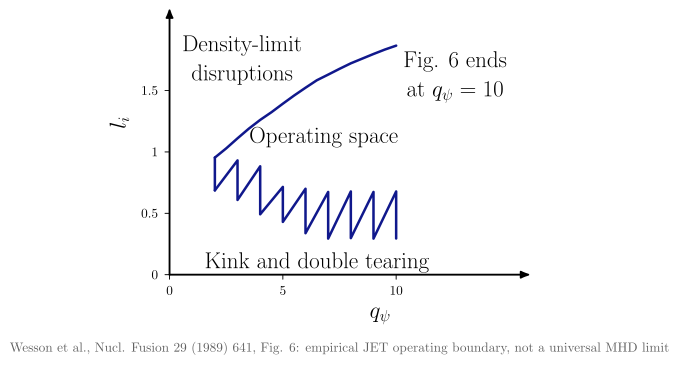
vaft.diagram.li_qa(reference='wesson_1989')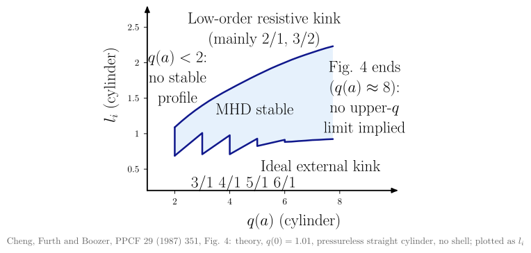
vaft.diagram.li_qa(reference='cheng_1987')The $l_i$-$q$ diagram of one source: Wesson 1989 (JET, empirical) or Cheng 1987 (theory).
vaft.diagram.li_qa(*, reference='wesson_1989', labels=True)Show source vaft/diagram/_li_qa.py, lines 68–135
def li_qa(*, reference: str = "wesson_1989", labels: bool = True) -> Diagram:
    r"""The $l_i$-$q$ diagram of one source: Wesson 1989 (JET, empirical) or Cheng 1987 (theory).

    Parameters
    ----------
    reference : {"wesson_1989", "cheng_1987"}
        Which published diagram. The two use different quantities: Wesson's
        $q_\psi$ and $l_i(3)$, Cheng's straight-cylinder $q(a)$ and $l_i$.
    labels : bool
        Draw region labels and the source note.

    Returns
    -------
    Diagram
        ``Diagram.model`` is a :class:`Chart` with the ``lower`` and ``upper``
        boundary curves in data coordinates and the projection key and
        boundary keys in ``parameters``.
    """
    try:
        spec = _REFERENCES[reference]
        spec = {**spec, "labels": dict(spec["labels"]), "text": dict(spec["text"])}   # never edit the table
    except KeyError:
        raise ValueError(f"reference must be one of {sorted(_REFERENCES)}, not {reference!r}") from None
    projection = get_projection(spec["projection"])
    chart = Chart(x_range=spec["x_range"], y_range=spec["y_range"])
    keys = []
    edges = []
    for key in projection.default_boundaries:
        boundary = _b.get_boundary(key)
        keys.append(key)
        if boundary.form == "threshold":  # a vertical q edge, drawn between the two branches below
            edges.append(boundary)
            continue
        lo, hi = boundary.applicability.ranges[boundary.input_names[0]]
        curve = _b.boundary_curve(boundary, boundary.input_names[0], _samples(lo, hi))
        xy = curve.xy[np.isfinite(curve.xy).all(axis=1)]
        # 9 decimals: the TikZ source (and the committed SVG's hash) must not depend on the platform's
        # last-bit floating-point differences, which flipped one printed coordinate (5.029 vs 5.0291)
        chart.curves[boundary.branch] = np.round(xy, 9)
    if reference == "cheng_1987":
        # the theoretical permissible domain, filled between the two bounds over the range Fig. 4 draws (#1603)
        lower, upper = chart.curves["lower"], chart.curves["upper"]
        top = np.interp(lower[:, 0], upper[:, 0], upper[:, 1], left=np.nan, right=np.nan)
        keep = np.isfinite(top)
        chart.curves["domain"] = np.round(np.vstack([lower[keep], np.c_[lower[keep, 0], top[keep]][::-1]]), 9)
        # the jig-saw edges at integer q(a) = m, where an m/1 resonance enters the plasma (comparison theorem, p. 354)
        for m in (3, 4, 5, 6):
            spec["labels"][f"m{m}"] = (m, 0.30)
            spec["text"][f"m{m}"] = f"${m}/1$"
    for boundary in edges:
        q_edge = float(_b.boundary_value(boundary))
        span = sorted(float(np.interp(q_edge, *chart.curves[b].T)) for b in ("lower", "upper"))
        chart.curves["edge"] = _b.threshold_curve(boundary, projection.y, span, target_axis="x").xy
    chart.labels.update(spec["labels"])
    chart.parameters.update({"reference": reference, "projection": projection.key, "boundaries": tuple(keys)})
    x_hi, y_hi = chart.x_range[1], chart.y_range[1]
    scene = _render_chart(
        chart,
        x_label=spec["x_label"],
        y_label=spec["y_label"],
        curve_styles={**({"domain": "region plasma"} if "domain" in chart.curves else {}),
                      **{name: "boundary" for name in ("lower", "upper", "edge") if name in chart.curves}},
        region_text=spec["text"] if labels else {},
        x_ticks=[t for t in _nice_ticks(x_hi) if t >= chart.x_range[0]],
        y_ticks=[t for t in _nice_ticks(y_hi) if t >= chart.y_range[0]],
        note=spec["note"] if labels else "",
    )
    return Diagram("li_qa", scene, model=chart)
Formats .svg .tex .pdf the SVG above is committed; build the others locally
import vaft.diagram

d = vaft.diagram.li_qa(reference='wesson_1989')
d.tikz  # the TikZ document as text
d.save("li_qa_wesson_1989.svg")  # rendered vector image, the canonical artifact; needs latex, dvisvgm
d.save("li_qa_wesson_1989.tex")  # the complete TikZ document, the text source
d.save("li_qa_wesson_1989.pdf")  # vector PDF; needs pdflatex
Single-particle motion diagrams: gyration and guiding-centre drifts
Module vaft.diagram._particle_motion
exb_drift
2 assets
source
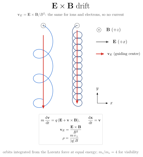
vaft.diagram.exb_drift()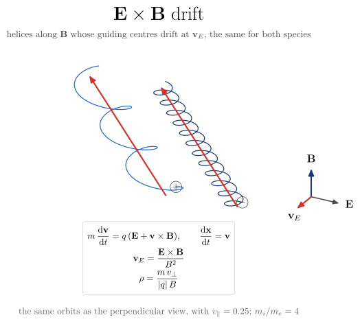
vaft.diagram.exb_drift(projection='3d')E-cross-B drift of an ion and an electron in uniform crossed fields.
vaft.diagram.exb_drift(*, mass_ratio=4.0, projection='perpendicular', labels=True)Show source vaft/diagram/_particle_motion.py, lines 149–223
def exb_drift(*, mass_ratio: float = 4.0, projection: str = "perpendicular", labels: bool = True) -> Diagram:
    r"""E-cross-B drift of an ion and an electron in uniform crossed fields.

    $\mathbf{B} = B\hat z$ (out of the page) and $\mathbf{E} = E\hat x$. Both
    particles have the same kinetic energy in their guiding-centre frames, so
    the ion's orbit is $\sqrt{m_i/m_e}$ times larger; both guiding centres
    move at the same ``exb_drift_velocity`` -- along $-\hat y$ -- so no
    current flows.

    ``projection="perpendicular"`` is the plane normal to $\mathbf{B}$;
    ``"3d"`` shows the same orbits with a small parallel velocity, as helices
    along $\mathbf{B}$ drifting sideways.
    """
    _check_projection(projection, ("perpendicular", "3d"))
    labels = _check_labels(labels)
    mass_ratio = _validate_mass_ratio(mass_ratio)
    E, B = np.array([0.2, 0.0, 0.0]), np.array([0.0, 0.0, 1.0])
    v_E = exb_drift_velocity(E, B)
    duration = 2.0 * math.pi * mass_ratio * 3.0  # three ion gyroperiods
    figure = ParticleFigure(parameters={"mass_ratio": mass_ratio, "E": float(E[0]), "B": float(B[2]),
                                        "duration": duration})
    rho_i = mass_ratio ** 0.5  # equal energy: u_i = u_e / sqrt(mass_ratio)
    gap = 2.2 * rho_i + 2.5
    for name, q, m, x_start in (("ion", 1.0, mass_ratio, 0.0), ("electron", -1.0, 1.0, gap)):
        u = 1.0 / math.sqrt(m)  # speed in the drift frame
        # start at the top of the orbit: gyration velocity along +x for an ion, -x for an electron
        u_vec = np.array([u * np.sign(q), 0.0, 0.0])
        x0 = np.array([x_start, 0.0, 0.0])
        v_par = np.array([0.0, 0.0, _EXB_V_PAR])
        x, _, dt = _orbit(q, m, x0, v_E + u_vec + v_par, _uniform(E), _uniform(B), 1.0,
                          duration / (2 * math.pi * m))
        figure.orbits[name] = x
        gc0 = _guiding_centre(q, m, x0, u_vec, B)
        figure.vectors[f"{name}_guiding_centre"] = gc0
        figure.vectors[f"{name}_drift"] = v_E
        figure.parameters[f"{name}_dt"] = dt
    figure.parameters["v_par"] = _EXB_V_PAR
    if projection == "3d":
        return _diagram("exb_drift_3d", _exb_3d(figure, labels), figure, labels)

    S = 0.45  # cm per unit length
    items: List = []
    for name, style in (("ion", "orbit ion"), ("electron", "orbit electron")):
        x = figure.orbits[name]
        items.append(Polyline.of(S * x[:, :2], style, role=f"{name}_orbit"))
        gc0 = figure.vectors[f"{name}_guiding_centre"]
        items.append(Arrow(tuple(S * gc0[:2]), tuple(S * (gc0 + v_E * duration)[:2]), "drift",
                           role=f"{name}_guiding_centre"))
        items.append(Label(tuple(S * x[0, :2]), "$+$" if name == "ion" else "$-$", "charge", role=f"{name}_start"))

    xs = np.concatenate([o[:, 0] for o in figure.orbits.values()])
    ys = np.concatenate([o[:, 1] for o in figure.orbits.values()])
    right, top, bottom = S * xs.max() + 1.3, S * ys.max(), S * ys.min()
    center = 0.5 * S * (xs.min() + xs.max()) + 1.2
    if labels:
        items += [
            Label((right + 0.25, top - 0.4), "$\\odot$", "legend symbol", role="legend"),
            Label((right + 0.8, top - 0.4), "$\\mathbf{B}$ ($+z$)", "label", anchor="west", role="legend"),
            Arrow((right, top - 1.5), (right + 1.2, top - 1.5), "field arrow", role="legend"),
            Label((right + 1.4, top - 1.5), "$\\mathbf{E}$ ($+x$)", "label", anchor="west", role="legend"),
            Label((right + 0.9, top - 2.6), "$\\mathbf{v}_E$ (guiding centre)", "small label", anchor="west",
                  role="legend"),
            Arrow((right, top - 2.6), (right + 0.8, top - 2.6), "drift", role="legend"),
            Arrow((right + 0.1, bottom + 0.4), (right + 1.1, bottom + 0.4), "axis", role="axes"),
            Label((right + 1.15, bottom + 0.4), "$x$", anchor="west", role="axes"),
            Arrow((right + 0.1, bottom + 0.4), (right + 0.1, bottom + 1.4), "axis", role="axes"),
            Label((right + 0.1, bottom + 1.45), "$y$", anchor="south", role="axes"),
        ]
        items += _title("$\\mathbf{E}\\times\\mathbf{B}$ drift",
                        "$\\mathbf{v}_E = \\mathbf{E}\\times\\mathbf{B}/B^2$: the same for ions and electrons, "
                        "so no current", top + 1.8, center)
        items.append(Label((center, bottom - 0.8),
                           f"orbits integrated from the Lorentz force at equal energy; "
                           f"$m_i/m_e = {mass_ratio:g}$ for visibility", "note", role="note"))
    return _diagram("exb_drift", Scene(tuple(items)), figure, labels)
Formats .svg .tex .pdf the SVG above is committed; build the others locally
import vaft.diagram

d = vaft.diagram.exb_drift()
d.tikz  # the TikZ document as text
d.save("exb_drift.svg")  # rendered vector image, the canonical artifact; needs latex, dvisvgm
d.save("exb_drift.tex")  # the complete TikZ document, the text source
d.save("exb_drift.pdf")  # vector PDF; needs pdflatex
Formula functions referenced:
particle.boris_orbit, particle.exb_drift_velocity, particle.gyration_offset, particle.gyrofrequency
curvature_drift
3 assets
source
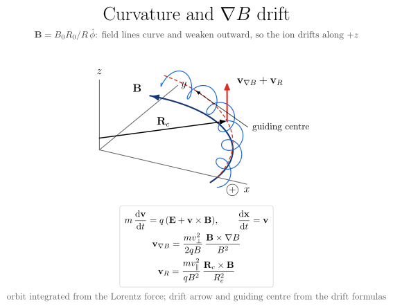
vaft.diagram.curvature_drift()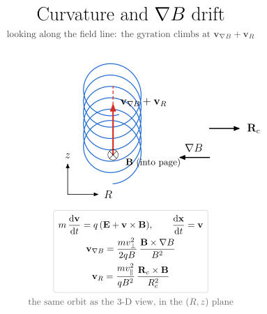
vaft.diagram.curvature_drift(projection='poloidal')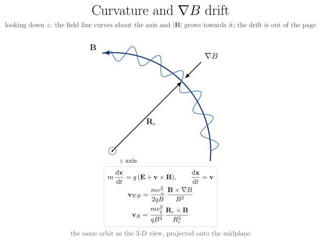
vaft.diagram.curvature_drift(projection='top')An ion spiralling along a curved field line and drifting off it.
vaft.diagram.curvature_drift(*, projection='3d', labels=True)Formats .svg .tex .pdf the SVG above is committed; build the others locally
import vaft.diagram

d = vaft.diagram.curvature_drift()
d.tikz  # the TikZ document as text
d.save("curvature_drift.svg")  # rendered vector image, the canonical artifact; needs latex, dvisvgm
d.save("curvature_drift.tex")  # the complete TikZ document, the text source
d.save("curvature_drift.pdf")  # vector PDF; needs pdflatex
Formula functions referenced:
equilibrium.vacuum_toroidal_field, particle.boris_orbit, particle.curvature_drift_velocity, particle.grad_b_drift_velocity, particle.gyration_offset, particle.gyrofrequency
magnetization_current
2 assets
source
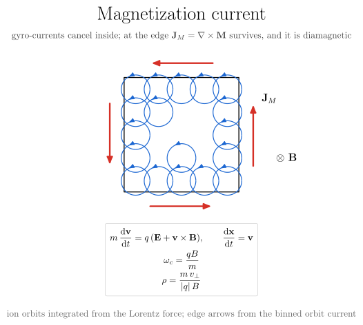
vaft.diagram.magnetization_current()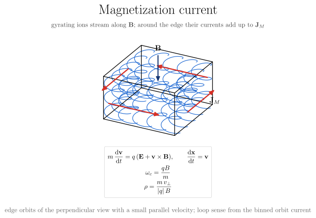
vaft.diagram.magnetization_current(projection='3d')Gyrating ions in a bounded region: interior currents cancel, the edge carries one.
vaft.diagram.magnetization_current(*, projection='perpendicular', labels=True)Formats .svg .tex .pdf the SVG above is committed; build the others locally
import vaft.diagram

d = vaft.diagram.magnetization_current()
d.tikz  # the TikZ document as text
d.save("magnetization_current.svg")  # rendered vector image, the canonical artifact; needs latex, dvisvgm
d.save("magnetization_current.tex")  # the complete TikZ document, the text source
d.save("magnetization_current.pdf")  # vector PDF; needs pdflatex
Formula functions referenced:
particle.boris_orbit, particle.gyrofrequency
toroidal_drift
3 assets
source
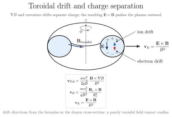
vaft.diagram.toroidal_drift()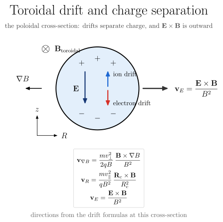
vaft.diagram.toroidal_drift(projection='poloidal')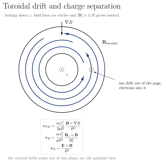
vaft.diagram.toroidal_drift(projection='top')Why a purely toroidal field cannot confine a plasma.
vaft.diagram.toroidal_drift(*, aspect_ratio=2.2, projection='3d', labels=True)Formats .svg .tex .pdf the SVG above is committed; build the others locally
import vaft.diagram

d = vaft.diagram.toroidal_drift()
d.tikz  # the TikZ document as text
d.save("toroidal_drift.svg")  # rendered vector image, the canonical artifact; needs latex, dvisvgm
d.save("toroidal_drift.tex")  # the complete TikZ document, the text source
d.save("toroidal_drift.pdf")  # vector PDF; needs pdflatex
Formula functions referenced:
equilibrium.vacuum_toroidal_field, particle.curvature_drift_velocity, particle.exb_drift_velocity, particle.grad_b_drift_velocity
Tearing physics upstream of the island: rational surface, Delta-prime, layer matching
Module vaft.diagram._tearing
rational_surface
1 asset
source
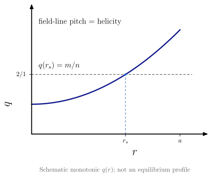
vaft.diagram.rational_surface()Where a helical perturbation resonates: the rational surface $q(r_s) = m/n$.
vaft.diagram.rational_surface(m=2, n=1, *, labels=True)Show source vaft/diagram/_tearing.py, lines 100–144
def rational_surface(m: int = 2, n: int = 1, *, labels: bool = True) -> Diagram:
    r"""Where a helical perturbation resonates: the rational surface $q(r_s) = m/n$.

    A schematic monotonic $q(r) = q_0 + (q_a - q_0)(r/a)^2$ -- not an
    equilibrium profile -- crosses the level $m/n$ exactly once, at $r_s$,
    where the field-line pitch matches the helicity of the $m/n$ perturbation.
    $m$ and $n$ are positive integers in lowest terms, as in ``magnetic_island``.
    """
    for name, value in (("m", m), ("n", n)):
        if isinstance(value, bool) or not isinstance(value, (int, np.integer)) or value <= 0:
            raise ValueError(f"{name} must be a positive integer mode number, not {value!r}")
    if math.gcd(int(m), int(n)) != 1:
        raise ValueError(f"m/n = {m}/{n} is not in lowest terms; use {m // math.gcd(m, n)}/{n // math.gcd(m, n)}")
    labels = _check_labels(labels)
    q_s = m / n
    q0, qa = _schematic_q(q_s)
    r_s = math.sqrt((q_s - q0) / (qa - q0))
    r = np.linspace(0.0, 1.0, 201)
    q = q0 + (qa - q0) * r**2
    chart = Chart(x_range=(0.0, 1.12), y_range=(0.0, 1.15 * qa))
    chart.curves["q_profile"] = np.stack([r, q], axis=-1)
    chart.curves["rational_level"] = np.array([[0.0, q_s], [1.08, q_s]])
    chart.curves["rational_surface"] = np.array([[r_s, 0.0], [r_s, q_s]])
    chart.points["crossing"] = (r_s, q_s)
    chart.parameters.update({"m": m, "n": n, "q_s": q_s, "q0": q0, "qa": qa, "r_s": r_s})
    # the y tick sits at q_s / (1.15 q_a); keep the axis title clear of it
    tick_height = q_s / chart.y_range[1]
    scene = render_chart(
        chart, x_label="$r$", y_label="$q$",
        curve_styles={"q_profile": "outer solution", "rational_level": "approx", "rational_surface": "rational"},
        region_text={},
        note="Schematic monotonic $q(r)$; not an equilibrium profile" if labels else "",
        x_ticks=(r_s, 1.0), x_tick_text=("$r_s$", "$a$"), y_ticks=(q_s,), y_tick_text=(f"${m}/{n}$",),
        y_label_at=0.25 if tick_height > 0.45 else 0.62,
    )
    crossing = Marker(tuple(chart.to_cm(chart.points["crossing"])), "o", "opoint", role="rational_surface")
    items = [crossing]
    if labels:
        at, anchor = _level_label_place(chart)
        items.append(Label(at, "$q(r_s) = m/n$", "label", anchor=anchor, role="rational_level"))
        # q < q_a * 0.3 + q_0 over the left third, so the top-left corner stays empty
        items.append(Label((0.25, CHART_HEIGHT - 0.1), "field-line pitch $=$ helicity", "label",
                           anchor="north west", role="region_pitch"))
        chart.parameters["level_label_anchor"] = anchor
    return Diagram("rational_surface", scene + Scene(tuple(items)), model=chart)
Formats .svg .tex .pdf the SVG above is committed; build the others locally
import vaft.diagram

d = vaft.diagram.rational_surface()
d.tikz  # the TikZ document as text
d.save("rational_surface.svg")  # rendered vector image, the canonical artifact; needs latex, dvisvgm
d.save("rational_surface.tex")  # the complete TikZ document, the text source
d.save("rational_surface.pdf")  # vector PDF; needs pdflatex
delta_prime
1 asset
source
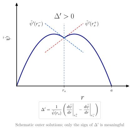
vaft.diagram.delta_prime()What $\Delta’$ measures: the slope jump of the outer solution across $r_s$.
vaft.diagram.delta_prime(sign='positive', *, labels=True)Show source vaft/diagram/_tearing.py, lines 182–232
def delta_prime(sign: str = "positive", *, labels: bool = True) -> Diagram:
    r"""What $\Delta'$ measures: the slope jump of the outer solution across $r_s$.

    Two schematic outer solutions -- one vanishing on the axis, one at the
    edge -- meet at $\tilde\psi(r_s)$ with different slopes; the dashed
    tangents show them. ``sign`` (``"positive"``, ``"zero"`` or
    ``"negative"``) sets the sign of the jump, and the index is evaluated by
    ``delta_prime_from_outer_derivatives`` from the drawn slopes. Only the
    sign is meaningful: this is not a stability calculation.
    """
    if not isinstance(sign, str):
        raise ValueError(f"sign must be one of {tuple(_SIGNS)}, not {sign!r}")
    branches = _outer_branches(sign)
    labels = _check_labels(labels)
    slope_minus, slope_plus = branches["slopes"]
    value = delta_prime_from_outer_derivatives(_PSI_S, slope_minus, slope_plus)
    chart = Chart(x_range=(0.0, 1.12), y_range=(0.0, 1.6))
    chart.curves.update({"outer_left": branches["outer_left"], "outer_right": branches["outer_right"],
                         "slope_left": _tangent(slope_minus), "slope_right": _tangent(slope_plus),
                         "rational_surface": np.array([[_R_S, 0.0], [_R_S, 1.3]])})
    chart.points["psi_s"] = (_R_S, _PSI_S)
    relation = {"positive": ">", "zero": "=", "negative": "<"}[sign]
    chart.parameters.update({"sign": sign, "r_s": _R_S, "psi_s": _PSI_S, "dpsi_dr_minus": slope_minus,
                             "dpsi_dr_plus": slope_plus, "delta_prime": value})
    scene = render_chart(
        chart, x_label="$r$", y_label="$\\tilde\\psi$",
        curve_styles={"rational_surface": "rational", "slope_left": "slope minus", "slope_right": "slope plus",
                      "outer_left": "outer solution", "outer_right": "outer solution"},
        region_text={},
        x_ticks=(_R_S, 1.0), x_tick_text=("$r_s$", "$a$"),
    )
    items = [Marker(tuple(chart.to_cm(chart.points["psi_s"])), "o", "opoint", role="psi_s")]
    if labels:
        top = chart.to_cm(np.array([_R_S, 1.46]))
        items.append(Label(tuple(top), f"$\\Delta' {relation} 0$", "region", role="delta_prime"))
        for key, text, default in (("slope_left", "$\\tilde\\psi'(r_s^-)$", 0),
                                   ("slope_right", "$\\tilde\\psi'(r_s^+)$", 1)):
            ends = chart.curves[key]
            # the upper end is clear of the outer curve, which lies under both tangents' tops
            index = default if ends[0, 1] == ends[1, 1] else int(np.argmax(ends[:, 1]))
            end = chart.to_cm(ends[index])
            dx, anchor = (-0.05, "east") if index == 0 else (0.05, "west")
            items.append(Label((float(end[0]) + dx, float(end[1])), text, "label", anchor=anchor, role=key))
    scene = scene + Scene(tuple(items))
    if labels:
        scene, below = _with_box(scene, f"$\\displaystyle {formula_equation(delta_prime_from_outer_derivatives)}$",
                                 -1.3)
        scene = scene + Scene((Label((CHART_WIDTH / 2, below - 0.45),
                                     "Schematic outer solutions; only the sign of $\\Delta'$ is meaningful",
                                     "note", anchor="north", role="note"),))
    return Diagram("delta_prime", scene, model=chart)
Formats .svg .tex .pdf the SVG above is committed; build the others locally
import vaft.diagram

d = vaft.diagram.delta_prime()
d.tikz  # the TikZ document as text
d.save("delta_prime.svg")  # rendered vector image, the canonical artifact; needs latex, dvisvgm
d.save("delta_prime.tex")  # the complete TikZ document, the text source
d.save("delta_prime.pdf")  # vector PDF; needs pdflatex
Formula functions referenced:
stability.delta_prime_from_outer_derivatives
tearing_layer_matching
1 asset
source
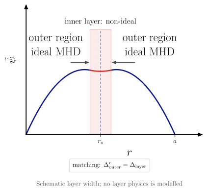
vaft.diagram.tearing_layer_matching()Why tearing theory splits the plasma into ideal outer regions and a thin inner layer.
vaft.diagram.tearing_layer_matching(*, labels=True)Show source vaft/diagram/_tearing.py, lines 249–304
def tearing_layer_matching(*, labels: bool = True) -> Diagram:
    r"""Why tearing theory splits the plasma into ideal outer regions and a thin inner layer.

    The outer solutions of ``delta_prime`` (the positive case) hold outside a
    layer of schematic half-width around $r_s$; inside, a non-ideal layer
    solution joins them, matching value and slope at both edges. The outer
    problem supplies $\Delta'$, the layer problem its own jump, and tearing
    stability follows from equating the two. No layer physics is modelled.
    """
    labels = _check_labels(labels)
    branches = _outer_branches("positive")
    lo, hi = _R_S - _LAYER_HALF_WIDTH, _R_S + _LAYER_HALF_WIDTH
    (A, B), (C, D) = branches["left_coefficients"], branches["right_coefficients"]
    left = branches["outer_left"][branches["outer_left"][:, 0] <= lo + 1e-12]
    right = branches["outer_right"][branches["outer_right"][:, 0] >= hi - 1e-12]
    left = np.vstack([left, [[lo, A * lo + B * lo**2]]]) if left[-1, 0] < lo else left
    right = np.vstack([[[hi, C * (1 - hi) + D * (1 - hi) ** 2]], right]) if right[0, 0] > hi else right
    inner = _hermite(lo, A * lo + B * lo**2, A + 2 * B * lo,
                     hi, C * (1 - hi) + D * (1 - hi) ** 2, -(C + 2 * D * (1 - hi)))
    y_top = 1.75
    chart = Chart(x_range=(0.0, 1.12), y_range=(0.0, 2.0))
    chart.curves.update({
        "outer_left": left, "outer_right": right, "inner_solution": inner,
        "inner_layer": np.array([[lo, 0.0], [hi, 0.0], [hi, y_top], [lo, y_top]]),
        "rational_surface": np.array([[_R_S, 0.0], [_R_S, y_top]]),
    })
    chart.labels.update({"outer_left": (0.2, 1.5), "outer_right": (0.83, 1.5)})
    chart.parameters.update({"r_s": _R_S, "layer_half_width": _LAYER_HALF_WIDTH, "layer_edges": (lo, hi)})
    region = {"outer_left": "outer region\\\\ ideal MHD", "outer_right": "outer region\\\\ ideal MHD"}
    scene = render_chart(
        chart, x_label="$r$", y_label="$\\tilde\\psi$",
        curve_styles={"rational_surface": "rational", "outer_left": "outer solution",
                      "outer_right": "outer solution", "inner_solution": "inner solution"},
        region_text=region if labels else {},
        x_ticks=(_R_S, 1.0), x_tick_text=("$r_s$", "$a$"),
    )
    band = Polyline.of(chart.to_cm(chart.curves["inner_layer"]), "layer", role="inner_layer", closed=True)
    items = [band]
    # the matching arrows run from each outer region to the layer edge it matches
    edge_y = 1.2
    for role, x_from, x_edge in (("matching_left", 0.3, lo), ("matching_right", 0.73, hi)):
        start = chart.to_cm(np.array([x_from, edge_y]))
        end = chart.to_cm(np.array([x_edge, edge_y]))
        items.append(Arrow(tuple(start), tuple(end), "match", role=role))
    if labels:
        top = chart.to_cm(np.array([_R_S, y_top]))
        items.append(Label((float(top[0]), float(top[1]) + 0.1),
                           "inner layer: non-ideal", "label", anchor="south", role="inner_layer"))
        items.append(Label((CHART_WIDTH / 2, -1.3),
                           "matching: $\\Delta'_{\\mathrm{outer}} = \\Delta_{\\mathrm{layer}}$",
                           "formula box", anchor="north", role="equations"))
        items.append(Label((CHART_WIDTH / 2, -2.4), "Schematic layer width; no layer physics is modelled",
                           "note", anchor="north", role="note"))
    # the band sits under the curves
    scene = Scene((band,) + scene.items + tuple(items[1:]))
    return Diagram("tearing_layer_matching", scene, model=chart)
Formats .svg .tex .pdf the SVG above is committed; build the others locally
import vaft.diagram

d = vaft.diagram.tearing_layer_matching()
d.tikz  # the TikZ document as text
d.save("tearing_layer_matching.svg")  # rendered vector image, the canonical artifact; needs latex, dvisvgm
d.save("tearing_layer_matching.tex")  # the complete TikZ document, the text source
d.save("tearing_layer_matching.pdf")  # vector PDF; needs pdflatex
3-D perturbation harmonics: what a complex Fourier coefficient means
Module vaft.diagram._harmonic
normal_field_component
1 asset
source
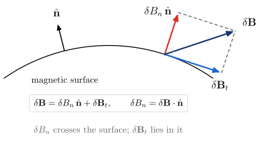
vaft.diagram.normal_field_component()$\delta B_n = \delta\mathbf B\cdot\hat{\mathbf n}$: the part of a perturbation that crosses a surface.
vaft.diagram.normal_field_component(*, labels=True)Show source vaft/diagram/_harmonic.py, lines 132–189
def normal_field_component(*, labels: bool = True) -> Diagram:
    r"""$\delta B_n = \delta\mathbf B\cdot\hat{\mathbf n}$: the part of a perturbation that crosses a surface.

    A perturbation $\delta\mathbf B$ at a point of a (schematic) magnetic
    surface splits into $\delta B_n\hat{\mathbf n}$ along the unit normal and
    $\delta\mathbf B_t$ in the surface. Only the normal part moves field
    lines off the surface; no code-specific normalisation is implied.
    """
    labels = _check_labels(labels)
    centre, radius = np.array([0.0, -6.0]), 7.0
    surface = _arc(radius, math.radians(55), math.radians(125), origin=tuple(centre), n=81)
    angle = math.radians(72)
    normal = np.array([math.cos(angle), math.sin(angle)])
    tangent = np.array([math.sin(angle), -math.cos(angle)])  # along the surface, to the right
    point = centre + radius * normal
    dB = 1.7 * normal + 2.3 * tangent  # [cm], schematic
    normal_part = float(dB @ normal) * normal
    tangential_part = dB - normal_part
    q_angle = math.radians(104)
    q_normal = np.array([math.cos(q_angle), math.sin(q_angle)])
    q_point = centre + radius * q_normal
    P = tuple(point)
    items: List = [
        Polyline.of(surface, "lcfs", role="surface"),
        Arrow(tuple(q_point), tuple(q_point + 1.1 * q_normal), "vector", role="surface_normal"),
        Polyline.of([point + normal_part, point + dB], "approx", role="construction"),
        Polyline.of([point + tangential_part, point + dB], "approx", role="construction"),
        Arrow(P, tuple(point + normal_part), "drift", role="normal_component"),
        Arrow(P, tuple(point + tangential_part), "drift ion", role="tangential_component"),
        Arrow(P, tuple(point + dB), "field vector", role="perturbation"),
    ]
    # right-angle mark between the normal and the surface
    s = 0.28
    items.append(Polyline.of([point + s * tangent, point + s * (tangent + normal), point + s * normal],
                             "surface", role="construction"))
    if labels:
        items += [
            Label(tuple(q_point + 1.25 * q_normal), "$\\hat{\\mathbf n}$", "label", anchor="south",
                  role="surface_normal"),
            Label(tuple(point + dB + 0.12 * (normal + tangent)), "$\\delta\\mathbf B$", "label",
                  anchor="south west", role="perturbation"),
            Label(tuple(point + normal_part - 0.15 * tangent), "$\\delta B_n\\,\\hat{\\mathbf n}$", "label",
                  anchor="east", role="normal_component"),
            Label(tuple(point + tangential_part - 0.2 * normal), "$\\delta\\mathbf B_t$", "label",
                  anchor="north", role="tangential_component"),
            Label(tuple(surface[-10] + np.array([0.1, -0.3])), "magnetic surface", "small label",
                  anchor="north west", role="surface"),
            _equation_box("$\\delta\\mathbf B = \\delta B_n\\,\\hat{\\mathbf n} + \\delta\\mathbf B_t,"
                          "\\qquad \\delta B_n = \\delta\\mathbf B\\cdot\\hat{\\mathbf n}$", 0.0, -0.9),
            _note("$\\delta B_n$ crosses the surface; $\\delta\\mathbf B_t$ lies in it", 0.0, -2.0),
        ]
    model = HarmonicFigure(
        vectors={"point": point, "normal": normal, "tangent": tangent, "perturbation": dB,
                 "normal_component": normal_part, "tangential_component": tangential_part,
                 "surface": surface, "surface_centre": centre},
        parameters={"surface_radius": radius, "delta_B_n": float(dB @ normal)},
    )
    return Diagram("normal_field_component", Scene(tuple(items)), model=model)
Formats .svg .tex .pdf the SVG above is committed; build the others locally
import vaft.diagram

d = vaft.diagram.normal_field_component()
d.tikz  # the TikZ document as text
d.save("normal_field_component.svg")  # rendered vector image, the canonical artifact; needs latex, dvisvgm
d.save("normal_field_component.tex")  # the complete TikZ document, the text source
d.save("normal_field_component.pdf")  # vector PDF; needs pdflatex
complex_harmonic
1 asset
source
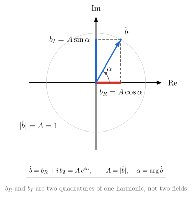
vaft.diagram.complex_harmonic()One harmonic as a complex coefficient $\hat b = b_R + i\,b_I = A\,e^{i\alpha}$.
vaft.diagram.complex_harmonic(amplitude=1.0, phase=1.0471975511965976, *, labels=True)Show source vaft/diagram/_harmonic.py, lines 234–292
def complex_harmonic(amplitude: float = 1.0, phase: float = math.pi / 3, *, labels: bool = True) -> Diagram:
    r"""One harmonic as a complex coefficient $\hat b = b_R + i\,b_I = A\,e^{i\alpha}$.

    The phasor's projections on the axes are $b_R = A\cos\alpha$ and
    $b_I = A\sin\alpha$, the cosine and sine quadratures of a single pattern;
    they are not two magnetic fields. The phasor is drawn at a fixed length
    and the circle it sweeps is labelled with the given amplitude.
    """
    A = _finite("amplitude", amplitude, positive=True)
    alpha = _wrapped(_finite("phase", phase))
    labels = _check_labels(labels)
    b = A * complex(math.cos(alpha), math.sin(alpha))
    unit = _UNIT / A
    tip = _xy(b, unit)
    # a quadrature this close to zero is drawn on an axis: its label moves off it
    eps = 0.08 * _UNIT
    items: List = _complex_axes(1.35 * _UNIT, labels=labels)
    items += [Polyline.of(_arc(_UNIT, 0.0, 2.0 * math.pi, n=121), "surface", role="amplitude", closed=True)]
    items += _quadratures(b, "construction", unit)
    items += [
        Polyline.of([(0.0, 0.0), (tip[0], 0.0)], "component real", role="real_component"),
        Polyline.of([(0.0, 0.0), (0.0, tip[1])], "component imag", role="imag_component"),
        Arrow((0.0, 0.0), tip, "phasor", role="phasor"),
        Marker(tip, "o", "opoint", role="phasor"),
    ]
    if abs(alpha) > 1e-9:
        items.append(Polyline.of(_arc(0.7, 0.0, alpha), "angle arc", role="phase"))
    if labels:
        direction = (math.cos(alpha), math.sin(alpha))
        diagonal = _diagonal_away_from(alpha, 0.0)
        circle_at = (1.02 * _UNIT * math.cos(diagonal), 1.02 * _UNIT * math.sin(diagonal))
        alpha_at = _clear_angle(0.0, alpha) if abs(alpha) >= 0.6 else alpha + math.copysign(0.35, alpha or 1.0)
        below = tip[1] >= -eps  # the b_R label goes on the side of the Re axis the phasor is not on
        items += [
            Label(tuple(np.array(tip) + 0.18 * np.array(direction)), "$\\hat b$", "label",
                  anchor=_outward_anchor(direction), role="phasor"),
            Label(circle_at, f"$|\\hat b| = A = {A:g}$", "label",
                  anchor=_outward_anchor((math.cos(diagonal), math.sin(diagonal))), role="amplitude"),
            Label((1.0 * math.cos(alpha_at), 1.0 * math.sin(alpha_at)), "$\\alpha$", "label",
                  anchor="center", role="phase"),
            Label((tip[0] if abs(tip[0]) > eps else 0.35, -0.2 if below else 0.2), "$b_R = A\\cos\\alpha$", "label",
                  anchor=("north" if below else "south") + ("" if abs(tip[0]) > eps else " west"),
                  role="real_component"),
            (Label((-0.2 if tip[0] >= -eps else 0.2, tip[1]), "$b_I = A\\sin\\alpha$", "label",
                   anchor="east" if tip[0] >= -eps else "west", role="imag_component") if abs(tip[1]) > eps
             # on the Re axis: below it, on the side the phasor is not
             else Label((-0.35 if tip[0] > 0 else 0.35, -0.25), "$b_I = A\\sin\\alpha$", "label",
                        anchor="north east" if tip[0] > 0 else "north west", role="imag_component")),
            _equation_box("$\\hat b = b_R + i\\,b_I = A\\,e^{i\\alpha}, \\qquad A = |\\hat b|,"
                          "\\quad \\alpha = \\arg\\hat b$", 0.0, -1.35 * _UNIT - 0.7),
            _note("$b_R$ and $b_I$ are two quadratures of one harmonic, not two fields",
                  0.0, -1.35 * _UNIT - 1.8),
        ]
    model = HarmonicFigure(
        vectors={"phasor": np.array(tip)},
        values={"b_hat": b},
        parameters={"amplitude": A, "phase": alpha, "real": b.real, "imag": b.imag, "cm_per_unit": unit},
    )
    return Diagram("complex_harmonic", Scene(tuple(items)), model=model)
Formats .svg .tex .pdf the SVG above is committed; build the others locally
import vaft.diagram

d = vaft.diagram.complex_harmonic()
d.tikz  # the TikZ document as text
d.save("complex_harmonic.svg")  # rendered vector image, the canonical artifact; needs latex, dvisvgm
d.save("complex_harmonic.tex")  # the complete TikZ document, the text source
d.save("complex_harmonic.pdf")  # vector PDF; needs pdflatex
toroidal_harmonic_phase
1 asset
source
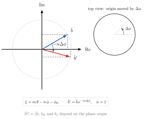
vaft.diagram.toroidal_harmonic_phase()The toroidal mode number is the rate at which the phase winds around the torus.
vaft.diagram.toroidal_harmonic_phase(n=1, *, labels=True)Show source vaft/diagram/_harmonic.py, lines 300–359
def toroidal_harmonic_phase(n: int = 1, *, labels: bool = True) -> Diagram:
    r"""The toroidal mode number is the rate at which the phase winds around the torus.

    Moving the toroidal origin by $\Delta\phi$ multiplies the coefficient by
    $e^{i\xi}$ with $\xi$ from ``helical_phase`` at $\theta = 0$, i.e. turns it
    by $-n\Delta\phi$ ($\Delta\phi = \pi/4$ here, so $n \le 7$ stays within one
    turn). The amplitude is unchanged; $b_R$ and $b_I$ are not, so they are
    meaningful only with a stated phase origin.
    """
    n = _mode("n", n)
    if n > _MAX_N:
        raise ValueError(f"n must be at most {_MAX_N} so the drawn rotation stays within one turn, not {n}")
    labels = _check_labels(labels)
    alpha0 = math.pi / 6
    b0 = complex(math.cos(alpha0), math.sin(alpha0))
    rotation = float(helical_phase(0.0, _DELTA_PHI, 1, n))  # = -n * delta_phi
    b1 = b0 * complex(math.cos(rotation), math.sin(rotation))
    arc_radius = 0.38 * _UNIT
    items: List = _complex_axes(1.35 * _UNIT, labels=labels)
    items += [Polyline.of(_arc(_UNIT, 0.0, 2.0 * math.pi, n=121), "surface", role="amplitude", closed=True)]
    items += _quadratures(b0, "construction", _UNIT) + _quadratures(b1, "construction", _UNIT)
    items += [
        Arrow((0.0, 0.0), _xy(b0), "phasor", role="phase_zero"),
        Arrow((0.0, 0.0), _xy(b1), "phasor alt", role="phase_shifted"),
        Polyline.of(_arc(arc_radius, alpha0, alpha0 + rotation, n=64), "angle arc", role="phasor"),
    ]
    # the toroidal angle, seen from above
    c, r = (2.45 * _UNIT, 0.5 * _UNIT), 0.7 * _UNIT
    items += [
        Polyline.of(_arc(r, 0.0, 2.0 * math.pi, origin=c, n=121), "lcfs", role="toroidal_angle", closed=True),
        Polyline.of([c, (c[0] + r, c[1])], "surface", role="toroidal_angle"),
        Polyline.of([c, (c[0] + r * math.cos(_DELTA_PHI), c[1] + r * math.sin(_DELTA_PHI))], "surface",
                    role="toroidal_angle"),
        Polyline.of(_arc(0.45 * r, 0.0, _DELTA_PHI, origin=c), "angle arc", role="toroidal_angle"),
    ]
    if labels:
        at = _clear_angle(alpha0, alpha0 + rotation, avoid=(alpha0, alpha0 + rotation))
        for value, text, role in ((b0, "$\\hat b$", "phase_zero"), (b1, "$\\hat b'$", "phase_shifted")):
            direction = (value.real, value.imag)
            items.append(Label(tuple(np.array(_xy(value)) + 0.18 * np.array(direction)), text, "label",
                               anchor=_outward_anchor(direction), role=role))
        items += [
            Label((0.62 * _UNIT * math.cos(at), 0.62 * _UNIT * math.sin(at)), "$-n\\Delta\\phi$",
                  "label", anchor="center", role="phasor"),
            Label((c[0] + 0.72 * r * math.cos(_DELTA_PHI / 2), c[1] + 0.72 * r * math.sin(_DELTA_PHI / 2)),
                  "$\\Delta\\phi$", "small label", anchor="center", role="toroidal_angle"),
            Label((c[0], c[1] + r + 0.15), "top view: origin moved by $\\Delta\\phi$", "small label",
                  anchor="south", role="toroidal_angle"),
            _equation_box(f"$\\displaystyle {formula_equation(helical_phase)}, \\qquad "
                          f"\\hat b' = \\hat b\\,e^{{-in\\Delta\\phi}},\\quad n = {n}$",
                          0.8 * _UNIT, -1.35 * _UNIT - 0.7),
            _note("$|\\hat b'| = |\\hat b|$; $b_R$ and $b_I$ depend on the phase origin",
                  0.8 * _UNIT, -1.35 * _UNIT - 1.8),
        ]
    model = HarmonicFigure(
        vectors={"phase_zero": np.array(_xy(b0)), "phase_shifted": np.array(_xy(b1))},
        values={"phase_zero": b0, "phase_shifted": b1},
        parameters={"n": n, "delta_phi": _DELTA_PHI, "rotation": rotation},
    )
    return Diagram("toroidal_harmonic_phase", Scene(tuple(items)), model=model)
Formats .svg .tex .pdf the SVG above is committed; build the others locally
import vaft.diagram

d = vaft.diagram.toroidal_harmonic_phase()
d.tikz  # the TikZ document as text
d.save("toroidal_harmonic_phase.svg")  # rendered vector image, the canonical artifact; needs latex, dvisvgm
d.save("toroidal_harmonic_phase.tex")  # the complete TikZ document, the text source
d.save("toroidal_harmonic_phase.pdf")  # vector PDF; needs pdflatex
Formula functions referenced:
stability.helical_phase
harmonic_real_space_projection
1 asset
source
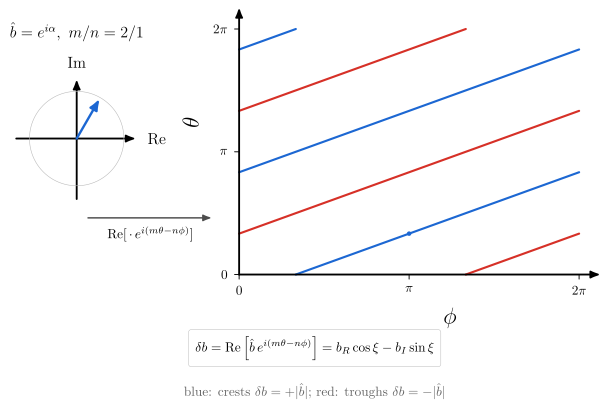
vaft.diagram.harmonic_real_space_projection()From a complex coefficient to the real field it stands for, $\mathrm{Re}[\hat b\,e^{i(m\theta - n\phi)}]$.
vaft.diagram.harmonic_real_space_projection(m=2, n=1, phase=1.0471975511965976, *, labels=True)Show source vaft/diagram/_harmonic.py, lines 377–437
def harmonic_real_space_projection(m: int = 2, n: int = 1, phase: float = math.pi / 3, *,
                                   labels: bool = True) -> Diagram:
    r"""From a complex coefficient to the real field it stands for, $\mathrm{Re}[\hat b\,e^{i(m\theta - n\phi)}]$.

    On the unwrapped $(\phi, \theta)$ plane the field of one harmonic with
    $\hat b = e^{i\alpha}$ is a set of parallel stripes of slope $n/m$; crests
    ($\delta b = +|\hat b|$) lie on $\xi = -\alpha$ and troughs on
    $\xi = \pi - \alpha$, evaluated by ``helical_harmonic``. Changing
    $\alpha$ slides the pattern; the complex number is its amplitude and
    position, the stripes are the physical field.
    """
    m, n = _mode("m", m), _mode("n", n)
    alpha = _wrapped(_finite("phase", phase))
    labels = _check_labels(labels)
    b = complex(math.cos(alpha), math.sin(alpha))
    two_pi = 2.0 * math.pi
    chart = Chart(x_range=(0.0, two_pi), y_range=(0.0, two_pi))
    crests = [line for line in _level_lines(m, n, -alpha) if clip(line, chart)]
    troughs = [line for line in _level_lines(m, n, math.pi - alpha) if clip(line, chart)]
    for i, line in enumerate(crests):
        chart.curves[f"crest_{i}"] = line
    for i, line in enumerate(troughs):
        chart.curves[f"trough_{i}"] = line
    # a crest point inside the box, checked against the formula
    sample = next(p for line in crests for p in line[len(line) // 2::7] if 0.3 < p[1] < two_pi - 0.3)
    chart.points["sample"] = (float(sample[0]), float(sample[1]))
    chart.parameters.update({"m": m, "n": n, "phase": alpha,
                             "sample_value": helical_harmonic(b, sample[1], sample[0], m, n)})
    ticks = (0.0, math.pi, two_pi)
    tick_text = ("$0$", "$\\pi$", "$2\\pi$")
    scene = render_chart(
        chart, x_label="$\\phi$", y_label="$\\theta$",
        curve_styles={**{f"crest_{i}": "crest" for i in range(len(crests))},
                      **{f"trough_{i}": "trough" for i in range(len(troughs))}},
        region_text={}, x_ticks=ticks, y_ticks=ticks, x_tick_text=tick_text, y_tick_text=tick_text,
    )
    # the curves carry numbered roles; give them the family role the tests and readers use
    items = [
        Polyline(it.points, it.style, "spatial_pattern", it.closed) if isinstance(it, Polyline)
        and it.role.startswith(("crest_", "trough_")) else it
        for it in scene.items
    ]
    items.append(Marker(tuple(chart.to_cm(np.array(chart.points["sample"]))), "o", "opoint",
                        role="real_projection"))
    # the coefficient, on its own complex plane to the left
    origin, unit = (-4.3, 3.6), 1.25
    items += _complex_axes(1.6, origin=origin, labels=labels)
    items += [Polyline.of(_arc(unit, 0.0, 2.0 * math.pi, origin=origin, n=97), "surface",
                          role="complex_coefficient", closed=True),
              Arrow(origin, _xy(b, unit, origin), "phasor", role="complex_coefficient"),
              Arrow((origin[0] + 0.3, origin[1] - 2.1), (-0.7, origin[1] - 2.1), "match", role="phase_factor")]
    if labels:
        items += [
            Label((origin[0], origin[1] + 2.45), f"$\\hat b = e^{{i\\alpha}},\\ m/n = {m}/{n}$", "label",
                  anchor="south", role="complex_coefficient"),
            Label((0.5 * (origin[0] - 0.4), origin[1] - 2.2), "$\\mathrm{Re}[\\,\\cdot\\,e^{i(m\\theta - n\\phi)}]$",
                  "small label", anchor="north", role="phase_factor"),
            _equation_box(f"$\\displaystyle {formula_equation(helical_harmonic)}$", 2.0, -1.45),
            _note("blue: crests $\\delta b = +|\\hat b|$; red: troughs $\\delta b = -|\\hat b|$", 2.0, -2.75),
        ]
    return Diagram("harmonic_real_space_projection", Scene(tuple(items)), model=chart)
Formats .svg .tex .pdf the SVG above is committed; build the others locally
import vaft.diagram

d = vaft.diagram.harmonic_real_space_projection()
d.tikz  # the TikZ document as text
d.save("harmonic_real_space_projection.svg")  # rendered vector image, the canonical artifact; needs latex, dvisvgm
d.save("harmonic_real_space_projection.tex")  # the complete TikZ document, the text source
d.save("harmonic_real_space_projection.pdf")  # vector PDF; needs pdflatex
Formula functions referenced:
stability.helical_harmonic
complex_field_superposition
1 asset
source
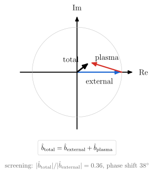
vaft.diagram.complex_field_superposition()External and plasma-response fields add as complex numbers.
vaft.diagram.complex_field_superposition(case='screening', *, labels=True)Show source vaft/diagram/_harmonic.py, lines 465–507
def complex_field_superposition(case: str = "screening", *, labels: bool = True) -> Diagram:
    r"""External and plasma-response fields add as complex numbers.

    $\hat b_\mathrm{total} = \hat b_\mathrm{external} + \hat b_\mathrm{plasma}$
    is a vector sum in the complex plane: a response opposing the external
    field screens it (``"screening"``), one nearly in phase amplifies it
    (``"amplification"``), and in general both size and phase change
    (``"phase_shift"``). The values are schematic, not a response calculation.
    """
    if not isinstance(case, str) or case not in _CASES:
        raise ValueError(f"case must be one of {tuple(_CASES)}, not {case!r}")
    labels = _check_labels(labels)
    external = complex(1.0, 0.0)
    plasma = complex(_CASES[case])
    total = external + plasma
    unit = 2.4
    extent = 1.1 * unit * max(abs(external), abs(total), 1.0) + 0.4
    origin, ext_tip, tot_tip = (0.0, 0.0), _xy(external, unit), _xy(total, unit)
    items: List = _complex_axes(extent, labels=labels)
    items += [
        Polyline.of(_arc(unit * abs(external), 0.0, 2.0 * math.pi, n=121), "surface", role="external",
                    closed=True),
        Arrow(origin, ext_tip, "phasor", role="external"),
        Arrow(ext_tip, tot_tip, "phasor alt", role="plasma"),
        Arrow(origin, tot_tip, "phasor total", role="total"),
    ]
    if labels:
        centroid = (np.array(origin) + np.array(ext_tip) + np.array(tot_tip)) / 3.0
        # the external arrow lies on the Re axis: label it below, the side the triangle is not on
        below = (0.0, 1.0) if tot_tip[1] >= 0 else (0.0, -1.0)
        items += [
            _side_label(origin, ext_tip, "external", below, "external"),
            _plasma_label(ext_tip, tot_tip, centroid, beyond=case == "amplification"),
            _side_label(origin, tot_tip, "total", centroid, "total"),
            _equation_box("$\\hat b_\\mathrm{total} = \\hat b_\\mathrm{external} + \\hat b_\\mathrm{plasma}$",
                          0.0, -extent - 0.6),
            _note(f"{case.replace('_', ' ')}: $|\\hat b_\\mathrm{{total}}|/|\\hat b_\\mathrm{{external}}|"
                  f" = {abs(total) / abs(external):.2f}$, phase shift "
                  f"${math.degrees(math.atan2(total.imag, total.real)):.0f}^\\circ$", 0.0, -extent - 1.6),
        ]
    model = HarmonicFigure(values={"external": external, "plasma": plasma, "total": total},
                           parameters={"case": case, "cm_per_unit": unit})
    return Diagram("complex_field_superposition", Scene(tuple(items)), model=model)
Formats .svg .tex .pdf the SVG above is committed; build the others locally
import vaft.diagram

d = vaft.diagram.complex_field_superposition()
d.tikz  # the TikZ document as text
d.save("complex_field_superposition.svg")  # rendered vector image, the canonical artifact; needs latex, dvisvgm
d.save("complex_field_superposition.tex")  # the complete TikZ document, the text source
d.save("complex_field_superposition.pdf")  # vector PDF; needs pdflatex
Collision processes in fusion plasmas: a classification diagram
Module vaft.diagram._collision
collision_processes
1 asset
source
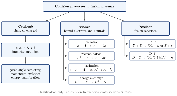
vaft.diagram.collision_processes()Collision processes in fusion plasmas: Coulomb, atomic and nuclear.
vaft.diagram.collision_processes(*, labels=True)Show source vaft/diagram/_collision.py, lines 66–120
def collision_processes(*, labels: bool = True) -> Diagram:
    r"""Collision processes in fusion plasmas: Coulomb, atomic and nuclear.

    Coulomb collisions (e--e, e--i, i--i, impurity--main ion) act through
    many small-angle deflections and relax the distribution: pitch-angle
    scattering, momentum exchange and energy equilibration. Atomic processes
    (ionization, recombination, excitation, charge exchange) change charge
    states or bound electrons. Nuclear reactions (D--D, D--T) change nuclei;
    the D--T alpha energy is ``vaft.formula.constants.E_ALPHA``. A
    classification, not a quantitative comparison.
    """
    labels = _check_labels(labels)
    items: List = []
    root = box(0.0, 0.0, 9.0, 1.1, "\\textbf{Collision processes in fusion plasmas}", role="collision",
               latex=True)
    items += list(root.items)
    branch_text = {
        "coulomb": "\\textbf{Coulomb}\\\\ charged--charged",
        "atomic": "\\textbf{Atomic}\\\\ bound electrons and neutrals",
        "nuclear": "\\textbf{Nuclear}\\\\ fusion reactions",
    }
    branches = {}
    for key, x in _BRANCH_X.items():
        b = box(x, _BRANCH_Y, _BRANCH_W, _BRANCH_H, branch_text[key], role=f"collision:{key}", latex=True)
        branches[key] = b
        items += list(b.items)
        items.append(connector(root, b, role=f"collision:{key}"))
    # Coulomb: who collides, then what the collisions do
    species = box(_BRANCH_X["coulomb"], _BRANCH_Y - 2.3, _BRANCH_W, 1.5,
                  "$e$--$e$, \\ $e$--$i$, \\ $i$--$i$\\\\ impurity--main ion",
                  role="collision:coulomb:species", latex=True)
    effects = box(_BRANCH_X["coulomb"], _BRANCH_Y - 4.9, _BRANCH_W, 2.0,
                  "pitch-angle scattering\\\\ momentum exchange\\\\ energy equilibration",
                  role="collision:coulomb:effects", latex=True)
    items += list(species.items) + list(effects.items)
    items += [connector(branches["coulomb"], species, role="collision:coulomb:species"),
              connector(species, effects, role="collision:coulomb:effects")]
    # atomic and nuclear: a spine of leaves under each branch
    for key, leaves in _leaves().items():
        parent = branches[key]
        x = parent.x + 0.75
        children = []
        for i, (role, text) in enumerate(leaves):
            y = _BRANCH_Y - 0.5 * _BRANCH_H - 0.9 - i * _ITEM_STEP
            child = box(x, y, _ITEM_W, _ITEM_H, text, style="concept leaf", role=role, latex=True)
            children.append(child)
            items += list(child.items)
        items += _spine(parent, children, role=f"collision:{key}")
    if labels:
        items.append(Label((0.0, _BRANCH_Y - 6.6),
                           "Classification only: no collision frequencies, cross-sections or rates",
                           "note", anchor="north", role="note"))
    model = {"branches": tuple(_BRANCH_X), "leaves": {k: tuple(r for r, _ in v) for k, v in _leaves().items()},
             "alpha_energy_MeV": _alpha_energy_MeV()}
    return Diagram("collision_processes", Scene(tuple(items)), model=model)
Formats .svg .tex .pdf the SVG above is committed; build the others locally
import vaft.diagram

d = vaft.diagram.collision_processes()
d.tikz  # the TikZ document as text
d.save("collision_processes.svg")  # rendered vector image, the canonical artifact; needs latex, dvisvgm
d.save("collision_processes.tex")  # the complete TikZ document, the text source
d.save("collision_processes.pdf")  # vector PDF; needs pdflatex
Geometric approximations: which geometry, which ordering, and how modes map
Module vaft.diagram._geometry
geometry_ordering_map
1 asset
source
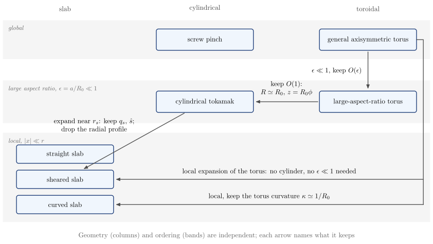
vaft.diagram.geometry_ordering_map()Geometry and ordering are two axes, not one hierarchy.
vaft.diagram.geometry_ordering_map(*, labels=True)Show source vaft/diagram/_geometry.py, lines 65–139
def geometry_ordering_map(*, labels: bool = True) -> Diagram:
    r"""Geometry and ordering are two axes, not one hierarchy.

    Columns are geometries (slab, cylindrical, toroidal), bands are orderings
    (global; large aspect ratio $\epsilon = a/R_0 \ll 1$; local). Each arrow is
    a reduction and names what it keeps or discards: the cylindrical tokamak
    is the $O(1)$ limit of a large-aspect-ratio torus, a local slab can come
    from the torus directly, and a curved slab keeps a $1/R_0$ curvature.
    """
    labels = _check_labels(labels)
    W = 5.0
    items: List = []
    left, right = -3.2, 18.8
    items += band(left, right, -1.0, 1.0, "global", role="ordering:global")
    items += band(left, right, -4.3, -2.1, "large aspect ratio, $\\epsilon = a/R_0 \\ll 1$",
                  role="ordering:large_aspect_ratio")
    items += band(left, right, -9.4, -4.8, "local, $|x| \\ll r$", role="ordering:local")
    for name, x in _COLUMNS.items():
        items.append(Label((x, 1.35), name, "subtitle", anchor="south", role=f"geometry:{name}"))
    col, row = _COLUMNS, _ROWS
    boxes = {
        "general_torus": box(col["toroidal"], row["global"], W, 1.1, "general axisymmetric torus",
                             role="representation:general_torus"),
        "screw_pinch": box(col["cylindrical"], row["global"], W, 1.1, "screw pinch",
                           role="representation:screw_pinch"),
        "lar_torus": box(col["toroidal"], row["large_aspect_ratio"], W, 1.1, "large-aspect-ratio torus",
                         role="representation:lar_torus"),
        "cyl_tokamak": box(col["cylindrical"], row["large_aspect_ratio"], W, 1.1, "cylindrical tokamak",
                           role="representation:cylindrical_tokamak"),
        "straight_slab": box(col["slab"], -5.9, W, 0.95, "straight slab", role="representation:straight_slab"),
        "sheared_slab": box(col["slab"], -7.2, W, 0.95, "sheared slab", role="representation:sheared_slab"),
        "curved_slab": box(col["slab"], -8.5, W, 0.95, "curved slab", role="representation:curved_slab"),
    }
    for b in boxes.values():
        items += list(b.items)
    # (start, end, label, position along the arrow, side: +1 left of travel, -1 right)
    paths = [
        ("general_torus", "lar_torus", "$\\epsilon \\ll 1$, keep $O(\\epsilon)$", 0.5, -1),
        ("lar_torus", "cyl_tokamak", "keep $O(1)$:\\\\ $R \\simeq R_0$, $z = R_0\\phi$", 0.5, -1),
        ("cyl_tokamak", "sheared_slab", "expand near $r_s$: keep $q_s$, $\\hat s$;\\\\ drop the radial profile",
         0.45, -1),
    ]
    for start, end, text, t, side in paths:
        arrow = connector(boxes[start], boxes[end], role=f"path:{start}->{end}")
        items.append(arrow)
        if labels:
            a0, a1 = np.array(arrow.start), np.array(arrow.end)
            d = (a1 - a0) / np.linalg.norm(a1 - a0)
            normal = side * np.array([-d[1], d[0]])
            at = a0 + t * (a1 - a0) + 0.2 * normal
            items.append(Label(tuple(at), text, "small label,align=center", anchor=_anchor_from(normal),
                               role=f"path:{start}->{end}"))
    # the torus reaches the local slabs directly -- locality, not aspect ratio, defines them.
    # The route runs down the right margin and along the local band, clear of every box.
    lane = right - 0.35
    general = boxes["general_torus"]
    items.append(Polyline.of([(general.x + 0.5 * general.width, general.y), (lane, general.y),
                              (lane, boxes["curved_slab"].y)], "connector line",
                             role="path:general_torus->local"))
    for name, text in (("sheared_slab", "local expansion of the torus: no cylinder, no $\\epsilon \\ll 1$ needed"),
                       ("curved_slab", "local, keep the torus curvature $\\kappa \\simeq 1/R_0$")):
        target = boxes[name]
        end = (target.x + 0.5 * target.width + 0.08, target.y)
        items.append(Arrow((lane, target.y), end, "connector", role=f"path:general_torus->{name}"))
        if labels:
            items.append(Label((0.5 * (lane + end[0]), target.y + 0.12), text, "small label", anchor="south",
                               role=f"path:general_torus->{name}"))
    paths += [("general_torus", "sheared_slab", "", 0, 0), ("general_torus", "curved_slab", "", 0, 0)]
    if labels:
        items.append(Label((0.5 * (left + right), -9.8),
                           "Geometry (columns) and ordering (bands) are independent; each arrow names what it keeps",
                           "note", anchor="north", role="note"))
    model = {"columns": dict(_COLUMNS), "boxes": {k: (b.x, b.y) for k, b in boxes.items()},
             "paths": tuple((a, b) for a, b, *_ in paths)}
    return Diagram("geometry_ordering_map", Scene(tuple(items)), model=model)
Formats .svg .tex .pdf the SVG above is committed; build the others locally
import vaft.diagram

d = vaft.diagram.geometry_ordering_map()
d.tikz  # the TikZ document as text
d.save("geometry_ordering_map.svg")  # rendered vector image, the canonical artifact; needs latex, dvisvgm
d.save("geometry_ordering_map.tex")  # the complete TikZ document, the text source
d.save("geometry_ordering_map.pdf")  # vector PDF; needs pdflatex
field_line_geometry
3 assets
source
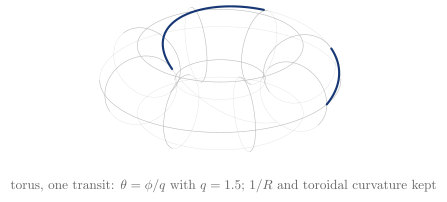
vaft.diagram.field_line_geometry(geometry='toroidal')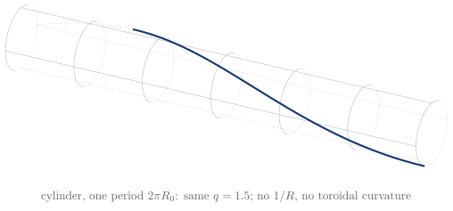
vaft.diagram.field_line_geometry(geometry='cylindrical')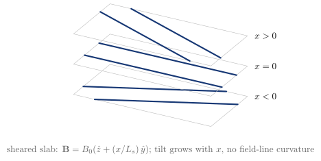
vaft.diagram.field_line_geometry(geometry='slab')The same field-line structure in toroidal, cylindrical and local sheared-slab geometry.
vaft.diagram.field_line_geometry(geometry='toroidal', *, labels=True)Show source vaft/diagram/_geometry.py, lines 248–269
def field_line_geometry(geometry: str = "toroidal", *, labels: bool = True) -> Diagram:
    r"""The same field-line structure in toroidal, cylindrical and local sheared-slab geometry.

    ``"toroidal"``: a straight field line $\theta = \phi/q$ on a circular
    surface of a torus. ``"cylindrical"``: the torus straightened at $R_0$,
    $z = R_0\phi$, with the same $q$ from ``cylindrical_safety_factor_from_r_B``.
    ``"slab"``: three planes of a sheared slab, field lines along
    ``sheared_slab_field``, their tilt growing with $x$. Each drops what its
    reduction discards: $1/R$ and curvature, then the global radius.
    """
    if geometry not in GEOMETRIES:
        raise ValueError(f"geometry must be one of {GEOMETRIES}, not {geometry!r}")
    labels = _check_labels(labels)
    built = {"toroidal": _field_line_torus, "cylindrical": _field_line_cylinder,
             "slab": _field_line_slab}[geometry](labels)
    items: List = list(built["items"])
    if labels:
        xy = np.vstack([np.asarray(it.points) for it in items if hasattr(it, "points")])
        items.append(Label((float(xy[:, 0].mean()), float(xy[:, 1].min()) - 0.6), built["caption"], "note",
                           anchor="north", role="note"))
    model = {"geometry": geometry, "field_line": built["line"], "pitch": built["pitch"]}
    return Diagram(f"field_line_geometry_{geometry}", Scene(tuple(items)), model=model)
Formats .svg .tex .pdf the SVG above is committed; build the others locally
import vaft.diagram

d = vaft.diagram.field_line_geometry(geometry='toroidal')
d.tikz  # the TikZ document as text
d.save("field_line_geometry_toroidal.svg")  # rendered vector image, the canonical artifact; needs latex, dvisvgm
d.save("field_line_geometry_toroidal.tex")  # the complete TikZ document, the text source
d.save("field_line_geometry_toroidal.pdf")  # vector PDF; needs pdflatex
Formula functions referenced:
geometry.cylindrical_safety_factor_from_r_B, geometry.sheared_slab_field
mode_number_mapping
1 asset
source
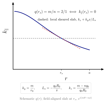
vaft.diagram.mode_number_mapping()$(m, n) \to (k_y, k_z)$: the rational surface is where $k_\parallel = 0$.
vaft.diagram.mode_number_mapping(m=2, n=1, *, labels=True)Show source vaft/diagram/_geometry.py, lines 277–332
def mode_number_mapping(m: int = 2, n: int = 1, *, labels: bool = True) -> Diagram:
    r"""$(m, n) \to (k_y, k_z)$: the rational surface is where $k_\parallel = 0$.

    $k_\parallel(r)$ of the $m/n$ harmonic in a cylinder with a schematic
    monotonic $q(r)$ (``cylindrical_parallel_wavenumber``) crosses zero at
    $q(r_s) = m/n$; the field-aligned local slab of ``local_slab_from_cylinder``
    is its tangent there, $k_\parallel \simeq k_z + k_y x/L_s$ with $x = r - r_s$
    and $k_z = 0$.
    """
    for name, value in (("m", m), ("n", n)):
        if isinstance(value, bool) or not isinstance(value, (int, np.integer)) or value <= 0:
            raise ValueError(f"{name} must be a positive integer mode number, not {value!r}")
    labels = _check_labels(labels)
    R0, a = 3.0, 1.0
    q_s = m / n
    q0, qa = _schematic_q(q_s)
    r = np.linspace(0.02, 1.0, 241) * a
    q = q0 + (qa - q0) * (r / a) ** 2
    r_s = a * math.sqrt((q_s - q0) / (qa - q0))
    s_hat = 2.0 * (qa - q0) * (r_s / a) ** 2 / q_s
    k_par = cylindrical_parallel_wavenumber(m, n, q, R0)
    k_y, L_s, k_z = local_slab_from_cylinder(m, n, r_s, R0, q_s, s_hat)
    span = float(np.max(np.abs(k_par)))
    chart = Chart(x_range=(0.0, 1.12 * a), y_range=(-1.15 * span, 1.15 * span))
    # the tangent, cut to the chart: at most a quarter radius each side, never past the axis
    slope = k_y / L_s
    reach = min(0.25 * a, r_s - 0.02 * a, 1.05 * span / abs(slope))
    x = np.array([-reach, 0.0, min(0.25 * a, 1.08 * a - r_s, 1.05 * span / abs(slope))])
    tangent = np.stack([r_s + x, sheared_slab_parallel_wavenumber(x, k_y, L_s, k_z)], axis=-1)
    chart.curves.update({"k_par": np.stack([r, k_par], axis=-1), "local_slab": tangent,
                         "zero": np.array([[0.0, 0.0], [1.08 * a, 0.0]])})
    chart.points["resonance"] = (r_s, 0.0)
    chart.parameters.update({"m": m, "n": n, "r_s": r_s, "q_s": q_s, "s_hat": s_hat, "R0": R0,
                             "k_y": k_y, "k_z": k_z, "L_s": L_s})
    scene = render_chart(
        chart, x_label="$r$", y_label="$k_\\parallel$",
        curve_styles={"zero": "approx", "k_par": "outer solution", "local_slab": "slope plus"},
        region_text={}, x_ticks=(r_s, a), x_tick_text=("$r_s$", "$a$"),
    )
    items: List = [Marker(tuple(chart.to_cm(chart.points["resonance"])), "o", "opoint", role="resonance")]
    if labels:
        curves = [chart.to_cm(chart.curves[k]) for k in ("k_par", "local_slab")]
        top = chart.to_cm(np.array([1.1 * a, 1.1 * span]))
        items.append(Label(tuple(top), f"$q(r_s) = m/n = {m}/{n} \\;\\Longleftrightarrow\\; k_\\parallel(r_s) = 0$",
                           "label", anchor="north east", role="resonance"))
        # outside r_s both the curve and the tangent are negative: the upper right stays empty
        under = chart.to_cm(np.array([1.1 * a, 0.8 * span]))
        items.append(Label(tuple(under), "dashed: local sheared slab, $k_z + k_y x/L_s$", "small label",
                           anchor="north east", role="local_slab"))
        items += [
            Label((CHART_WIDTH / 2, -1.4), f"$\\displaystyle {formula_equation(local_slab_from_cylinder)}$",
                  "formula box", anchor="north", role="equations"),
            Label((CHART_WIDTH / 2, -2.75), "Schematic $q(r)$; field-aligned slab at $r_s$, "
                  "$e^{i(m\\theta - n\\phi)}$", "note", anchor="north", role="note"),
        ]
    return Diagram("mode_number_mapping", scene + Scene(tuple(items)), model=chart)
Formats .svg .tex .pdf the SVG above is committed; build the others locally
import vaft.diagram

d = vaft.diagram.mode_number_mapping()
d.tikz  # the TikZ document as text
d.save("mode_number_mapping.svg")  # rendered vector image, the canonical artifact; needs latex, dvisvgm
d.save("mode_number_mapping.tex")  # the complete TikZ document, the text source
d.save("mode_number_mapping.pdf")  # vector PDF; needs pdflatex
Formula functions referenced:
geometry.cylindrical_parallel_wavenumber, geometry.local_slab_from_cylinder, geometry.sheared_slab_parallel_wavenumber
Reduced physical representations: how plasma information is compressed
Module vaft.diagram._reduced_representations
reduced_representation_hierarchy
1 asset
source
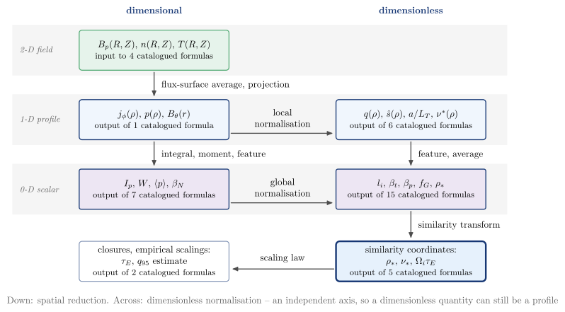
vaft.diagram.reduced_representation_hierarchy()Spatial reduction and dimensionless normalisation as two independent axes.
vaft.diagram.reduced_representation_hierarchy(*, labels=True)Show source vaft/diagram/_reduced_representations.py, lines 88–99
def reduced_representation_hierarchy(*, labels: bool = True) -> Diagram:
    r"""Spatial reduction and dimensionless normalisation as two independent axes.

    Rows are the output representation (2-D field, 1-D profile, 0-D scalar),
    columns dimensional and dimensionless: a local $\nu^*(\rho)$ is a
    dimensionless *profile*, a global $\beta$ a dimensionless *scalar*.
    Below them, similarity coordinates and closures / empirical scalings. Each
    cell gives examples and the number of catalogued formulas whose
    ``Reduction`` section outputs there, the column decided by the formula's
    documented return unit (``-`` is dimensionless).
    """
    return _hierarchy("reduced_representation_hierarchy", labels=labels, compact=False)
Formats .svg .tex .pdf the SVG above is committed; build the others locally
import vaft.diagram

d = vaft.diagram.reduced_representation_hierarchy()
d.tikz  # the TikZ document as text
d.save("reduced_representation_hierarchy.svg")  # rendered vector image, the canonical artifact; needs latex, dvisvgm
d.save("reduced_representation_hierarchy.tex")  # the complete TikZ document, the text source
d.save("reduced_representation_hierarchy.pdf")  # vector PDF; needs pdflatex
Formula functions referenced:
catalog.list_formulas
reduced_representation_hierarchy_compact
1 asset
source
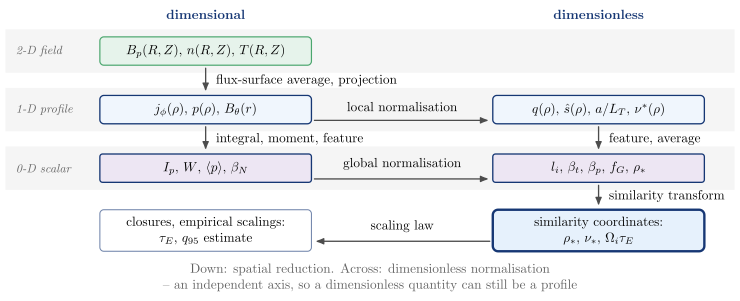
vaft.diagram.reduced_representation_hierarchy_compact()The two-axis representation hierarchy with symbols only, compactly spaced.
vaft.diagram.reduced_representation_hierarchy_compact(*, labels=True)Show source vaft/diagram/_reduced_representations.py, lines 102–113
def reduced_representation_hierarchy_compact(*, labels: bool = True) -> Diagram:
    r"""The two-axis representation hierarchy with symbols only, compactly spaced.

    The same rows (2-D field, 1-D profile, 0-D scalar, then similarity
    coordinates and closures / empirical scalings), columns (dimensional,
    dimensionless) and arrows (flux-surface average, integral, local and
    global normalisation, similarity transform, scaling law) as
    :func:`reduced_representation_hierarchy`, without the catalogued-formula
    counts: each box carries only its example symbols, and the boxes and gaps
    are shorter.
    """
    return _hierarchy("reduced_representation_hierarchy_compact", labels=labels, compact=True)
Formats .svg .tex .pdf the SVG above is committed; build the others locally
import vaft.diagram

d = vaft.diagram.reduced_representation_hierarchy_compact()
d.tikz  # the TikZ document as text
d.save("reduced_representation_hierarchy_compact.svg")  # rendered vector image, the canonical artifact; needs latex, dvisvgm
d.save("reduced_representation_hierarchy_compact.tex")  # the complete TikZ document, the text source
d.save("reduced_representation_hierarchy_compact.pdf")  # vector PDF; needs pdflatex
Formula functions referenced:
catalog.list_formulas
reduction_graph
4 assets
source

vaft.diagram.reduction_graph(family='current_q')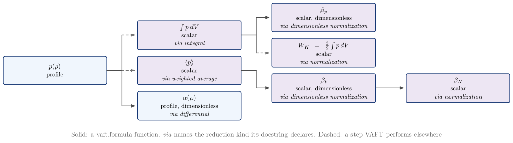
vaft.diagram.reduction_graph(family='pressure_energy')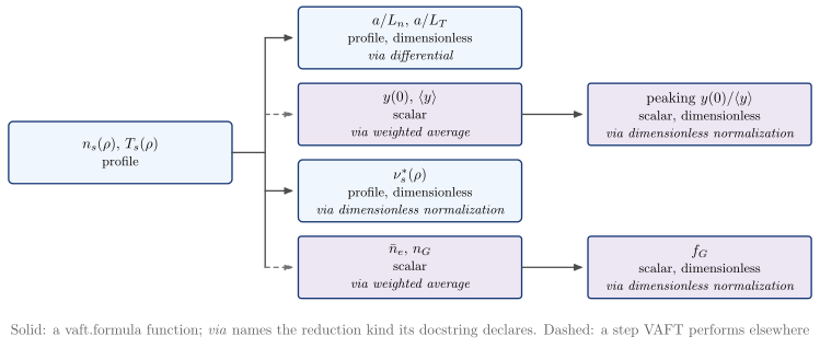
vaft.diagram.reduction_graph(family='kinetic_profiles')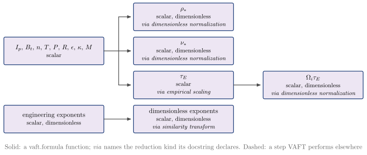
vaft.diagram.reduction_graph(family='dimensionless_similarity')One reduction family as a layered graph of quantities.
vaft.diagram.reduction_graph(family='current_q', *, labels=True)Formats .svg .tex .pdf the SVG above is committed; build the others locally
import vaft.diagram

d = vaft.diagram.reduction_graph(family='current_q')
d.tikz  # the TikZ document as text
d.save("reduction_graph_current_q.svg")  # rendered vector image, the canonical artifact; needs latex, dvisvgm
d.save("reduction_graph_current_q.tex")  # the complete TikZ document, the text source
d.save("reduction_graph_current_q.pdf")  # vector PDF; needs pdflatex
Formula functions referenced:
catalog.describe
How MHD mode families map across slab, cylindrical and toroidal geometry
Module vaft.diagram._mode_geometry
mhd_mode_geometry_map
1 asset
source
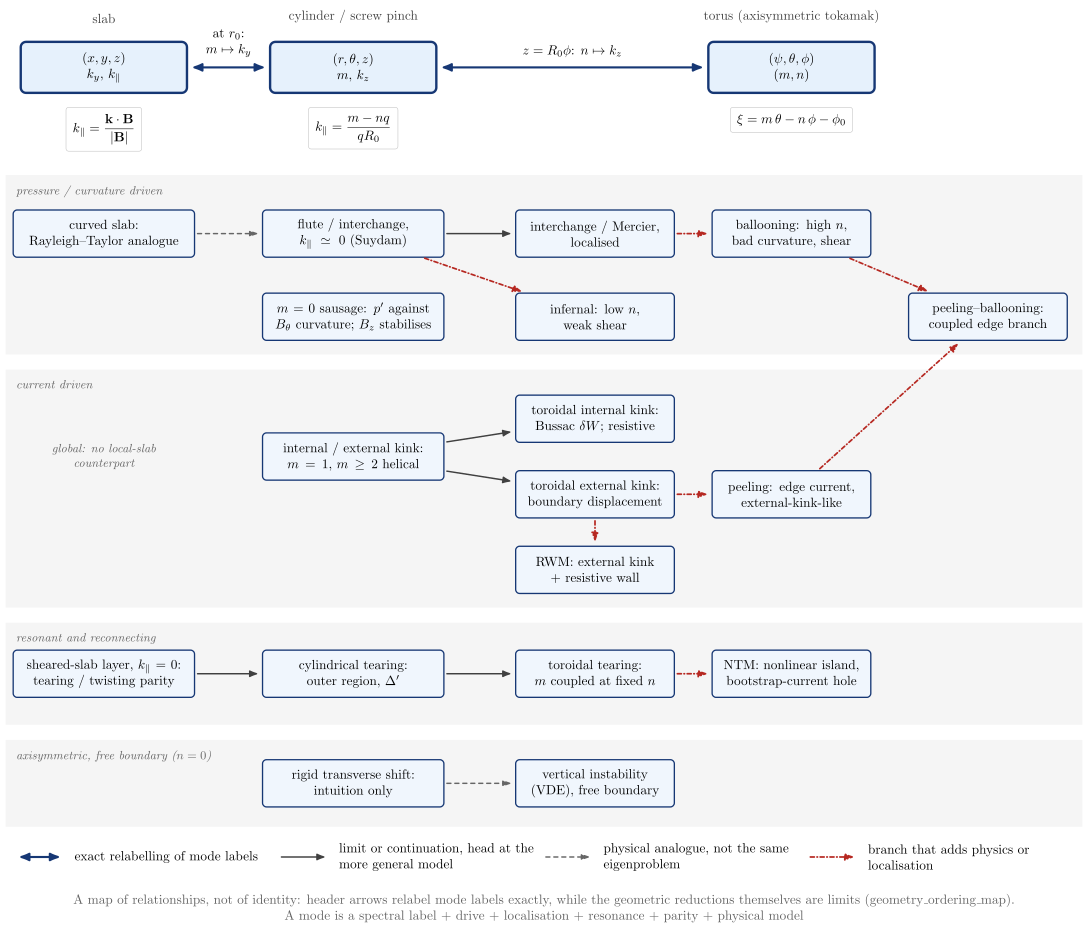
vaft.diagram.mhd_mode_geometry_map()MHD mode families across slab, cylindrical and toroidal geometry, with typed relations.
vaft.diagram.mhd_mode_geometry_map(*, labels=True)Show source vaft/diagram/_mode_geometry.py, lines 108–179
def mhd_mode_geometry_map(*, labels: bool = True) -> Diagram:
    r"""MHD mode families across slab, cylindrical and toroidal geometry, with typed relations.

    Columns are geometries, each headed by its coordinates, spectral labels
    and spectral relation: ``slab_parallel_wavenumber``,
    ``cylindrical_parallel_wavenumber`` ($k_\parallel = 0 \Leftrightarrow
    q = m/n$) and ``helical_phase``. The header arrows relabel mode labels
    exactly; the geometric reductions behind them are limits
    (``geometry_ordering_map``). Bands are physical families: pressure /
    curvature driven (Rayleigh--Taylor analogue, interchange, the $m = 0$
    sausage, Mercier,
    ballooning, infernal, peeling--ballooning), current driven (internal and
    external kink in the cylinder and the torus, peeling, RWM), resonant
    (layer parity, outer tearing, toroidal tearing, NTM) and the $n = 0$
    vertical instability. Arrows are typed: an exact relabelling, a limit or
    coordinate continuation, a physical analogue, or a branch that adds
    physics or localisation. A connection is a relationship, not identity.
    """
    labels = _check_labels(labels)
    left, right = -2.6, 25.9
    items: List = []
    for name, (top, bottom, text) in FAMILIES.items():
        items += band(left, right, bottom, top, text, role=f"family:{name}")
    titles = {"slab": (_SLAB, "slab"), "cylinder": (_CYL, "cylinder / screw pinch"),
              "torus": (_T2, "torus (axisymmetric tokamak)")}
    for name, (x, text) in titles.items():
        items.append(Label((x, 1.05), text, "subtitle", anchor="south", role=f"geometry:{name}"))
    nodes = {}
    for name, (x, y, family, text) in _NODES.items():
        width = 4.4 if family is None else (_W if x > _CYL else _W_LOCAL)
        style = "concept strong" if family is None else "concept box"
        nodes[name] = box(x, y, width, 1.35 if family is None else _H, text, style=style,
                          role=f"node:{name}", latex=True)
        items += list(nodes[name].items)
    # each geometry's resonance, from the catalog
    for name, (x, function) in {"slab": (_SLAB, slab_parallel_wavenumber),
                                "cylinder": (_CYL, cylindrical_parallel_wavenumber),
                                "torus": (_T2, helical_phase)}.items():
        items.append(Label((x, -1.05), f"$\\displaystyle {formula_equation(function)}$", "formula box",
                           anchor="north", role=f"equation:{name}"))
    for start, end, relation, text in _EDGES:
        arrow = connector(nodes[start], nodes[end], style=RELATIONS[relation][0],
                          role=f"edge:{relation}:{start}->{end}")
        items.append(arrow)
        if text:
            mid = 0.5 * (np.array(arrow.start) + np.array(arrow.end))
            items.append(Label((float(mid[0]), float(mid[1]) + 0.15), text, "small label,align=center", anchor="south",
                               role=f"edge:{relation}:{start}->{end}"))
    # global current-driven modes have no local-slab form
    items.append(Label((_SLAB, -10.3), "global: no local-slab\\\\ counterpart", "concept annotation",
                       role="note:no_slab_kink"))
    if labels:
        y = -20.9
        x0 = left + 0.3
        for i, (relation, (style, text)) in enumerate(RELATIONS.items()):
            x = x0 + 7.0 * i
            items.append(Arrow((x, y), (x + 1.2, y), style, role=f"legend:{relation}"))
            items.append(Label((x + 1.4, y), text, _LEGEND_STYLE, anchor="west", role=f"legend:{relation}"))
        items.append(Label((0.5 * (left + right), -21.75),
                           "A map of relationships, not of identity: header arrows relabel mode labels exactly, "
                           "while the geometric reductions themselves are limits (geometry\\_ordering\\_map).\\\\ "
                           "A mode is a "
                           "spectral label + drive + localisation + resonance + parity + physical model",
                           "note", anchor="north", role="note"))
    model = {
        "columns": dict(GEOMETRY_COLUMNS),
        "nodes": {k: (b.x, b.y) for k, b in nodes.items()},
        "families": {k: v[2] for k, v in _NODES.items() if v[2] is not None},
        "edges": tuple((a, b, rel) for a, b, rel, _ in _EDGES),
        "relations": {k: v[1] for k, v in RELATIONS.items()},
    }
    return Diagram("mhd_mode_geometry_map", Scene(tuple(items)), model=model)
Formats .svg .tex .pdf the SVG above is committed; build the others locally
import vaft.diagram

d = vaft.diagram.mhd_mode_geometry_map()
d.tikz  # the TikZ document as text
d.save("mhd_mode_geometry_map.svg")  # rendered vector image, the canonical artifact; needs latex, dvisvgm
d.save("mhd_mode_geometry_map.tex")  # the complete TikZ document, the text source
d.save("mhd_mode_geometry_map.pdf")  # vector PDF; needs pdflatex
Formula functions referenced:
geometry.cylindrical_parallel_wavenumber, geometry.slab_parallel_wavenumber, stability.helical_phase
Asymptotic orderings: the time and length scales a reduced model assumes (#1627, #1739)
Module vaft.diagram._orderings
timescale_hierarchy
1 asset
source
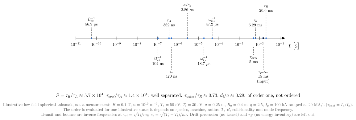
vaft.diagram.timescale_hierarchy()The timescales of one illustrative state on a logarithmic axis, with the ratios that order them.
vaft.diagram.timescale_hierarchy(*, labels=True)Show source vaft/diagram/_orderings.py, lines 118–192
def timescale_hierarchy(*, labels: bool = True) -> Diagram:
    r"""The timescales of one illustrative state on a logarithmic axis, with the ratios that order them.

    Inverse gyrofrequencies $1/\Omega$ (``particle.gyrofrequency``), the electron collision time
    (``ordering.braginskii_electron_collision_time``), the Alfven time over
    the minor radius, the sound crossing time ``a/c_s`` (``sol.ion_sound_speed``,
    $c_s = \\sqrt{(T_e + T_i)/m_i}$), the inverse thermal-ion transit and
    deeply-trapped bounce frequencies at $v_{ti} = \\sqrt{T_i/m_i}$
    (``neoclassical.transit_frequency``, ``deeply_trapped_bounce_frequency``;
    a period is $2\\pi$ times longer),
    the $I_p$-ramp evolution time, the thin-wall time
    (``vde.thin_wall_time``), the pulse (an input) and the resistive
    diffusion time from Spitzer resistivity. The drift precession has no
    formula kernel and $\tau_E$ needs an energy inventory the state does not
    carry; both are left out and the caption says so. The ratios below the axis --
    $S = \tau_R/\tau_A$, $\tau_{evol}/\tau_A$, $\tau_{pulse}/\tau_R$, $d_i/a$
    -- are the ordering parameters; the hierarchy is evaluated, not
    assumed.
    """
    labels = _check_labels(labels)
    times = timescales()
    items: List = []
    length = _DECADES * _DECADE
    items.append(Arrow((0.0, 0.0), (length + 0.5, 0.0), "chart axis", role="axis"))
    for k in range(_DECADES + 1):
        x = k * _DECADE
        items.append(Polyline.of([(x, -0.12), (x, 0.12)], "connector line", role="ticks"))
        items.append(Label((x, -0.25), f"$10^{{{int(_X0) + k}}}$", "ticklabel", anchor="north", role="ticks"))
    items.append(Label((length + 0.6, -0.25), "$t$ [s]", "xlabel", anchor="north west", role="axis"))
    order = sorted(times.items(), key=lambda kv: kv[1][1])
    placed, below = [], []
    for i, (key, (symbol, value, given)) in enumerate(order):
        x = _x(value)
        items.append(Marker((x, 0.0), "o", "opoint" if not given else "xpoint", role=f"time:{key}"))
        up = i % 2 == 0
        # stack labels that would collide with an earlier one on the same side: the first free level
        level = _free_level(placed, x, up, 3.4)
        placed.append((x, up, level))
        y = (0.9 + 1.25 * level) * (1 if up else -1) - (0.0 if up else 0.55)
        if not up:
            below.append(y)
        # below the axis the leader starts under the tick labels, so it never strikes through one
        items.append(Polyline.of([(x, 0.0 if up else -0.75), (x, y)], "approx", role=f"time:{key}"))
        if labels:
            text = f"{symbol}\\\\ {_fmt(value)}" + ("\\\\ (input)" if given else "")
            items.append(Label((x, y), text, "small label,align=center", anchor="south" if up else "north",
                               role=f"time:{key}"))
    s = ILLUSTRATIVE_STATE
    ratios = {
        "lundquist": times["resistive"][1] / times["alfven"][1],  # S = tau_R / tau_A at the same length
        "quasi_static": times["evolution"][1] / times["alfven"][1],
        "relaxation": times["pulse"][1] / times["resistive"][1],
        "hall": inertial_length(s["n"], MI_P) / s["a"],
    }
    lowest = min(below + [-0.75]) - 1.6   # under the deepest label (up to three lines tall)
    if labels:
        items.append(Label((0.5 * length, lowest - 0.3),
                           f"$S = \\tau_R/\\tau_A \\approx {_sci(ratios['lundquist'])}$, "
                           f"$\\tau_{{evol}}/\\tau_A \\approx {_sci(ratios['quasi_static'])}$: well separated. "
                           f"$\\tau_{{pulse}}/\\tau_R \\approx {ratios['relaxation']:.2g}$, "
                           f"$d_i/a \\approx {ratios['hall']:.2g}$: of order one, not ordered",
                           "label", anchor="north", role="ratios"))
        items.append(Label((0.5 * length, lowest - 1.1),
                           f"Illustrative low-field spherical tokamak, not a measurement: $B = {s['B']:g}$ T, "
                           f"$n = 10^{{19}}$ m$^{{-3}}$, $T_e = {s['T_e']:g}$ eV, $T_i = {s['T_i']:g}$ eV, "
                           f"$a = {s['a']:g}$ m, $R_0 = {s['R0']:g}$ m, $q = {s['q']:g}$, "
                           f"$I_p = 100$ kA ramped at $20$ MA/s ($\\tau_{{evol}} = I_p/\\dot I_p$).\\\\ "
                           "The order is evaluated for one illustrative state; it depends on species, machine, "
                           "radius, $T$, $B$, collisionality and mode frequency.\\\\ Transit and bounce are inverse "
                           "frequencies at $v_{ti} = \\sqrt{T_i/m_i}$; $c_s = \\sqrt{(T_e + T_i)/m_i}$. Drift "
                           "precession (no kernel) and $\\tau_E$ (no energy inventory) are left out.",
                           "note,align=center", anchor="north", role="note"))
    model = {"times": {k: v[1] for k, v in times.items()}, "inputs": {k for k, v in times.items() if v[2]},
             "ratios": ratios, "state": dict(ILLUSTRATIVE_STATE)}
    return Diagram("timescale_hierarchy", Scene(tuple(items)), model=model)
Formats .svg .tex .pdf the SVG above is committed; build the others locally
import vaft.diagram

d = vaft.diagram.timescale_hierarchy()
d.tikz  # the TikZ document as text
d.save("timescale_hierarchy.svg")  # rendered vector image, the canonical artifact; needs latex, dvisvgm
d.save("timescale_hierarchy.tex")  # the complete TikZ document, the text source
d.save("timescale_hierarchy.pdf")  # vector PDF; needs pdflatex
Formula functions referenced:
equilibrium.coulomb_logarithm_from_n_T, equilibrium.spitzer_resistivity_from_T_e_Z_eff_ln_Lambda, neoclassical.deeply_trapped_bounce_frequency, neoclassical.transit_frequency, ordering.alfven_time, ordering.braginskii_electron_collision_time, ordering.evolution_time, ordering.inertial_length, ordering.resistive_diffusion_time, ordering.thermal_speed, particle.gyrofrequency, sol.ion_sound_speed, stability.v_alfven_from_B_n_mi, vde.thin_wall_time
spatial_scale_orderings
1 asset
source
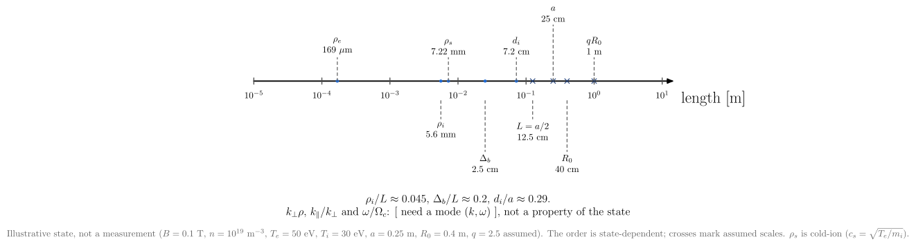
vaft.diagram.spatial_scale_orderings()The lengths of one illustrative state on a logarithmic axis, with the ratios that order them.
vaft.diagram.spatial_scale_orderings(*, labels=True)Show source vaft/diagram/_orderings.py, lines 221–282
def spatial_scale_orderings(*, labels: bool = True) -> Diagram:
    r"""The lengths of one illustrative state on a logarithmic axis, with the ratios that order them.

    Electron and ion Larmor radii (``particle.larmor_radius`` at the thermal
    speed), the sound gyroradius (``ordering.sound_gyroradius``), the ion
    skin depth (``ordering.inertial_length``), the ion banana width
    (``neoclassical.banana_width``), an illustrative gradient length $a/2$,
    the minor radius, the connection length $qR_0$ and $R_0$, all on the
    state of :func:`timescale_hierarchy`. Below the axis, the ordering ratios
    a length fixes ($\rho_i/L$, $d_i/a$, $\Delta_b/L$) and, as brackets, the
    ones that need a mode ($k_\perp\rho$, $k_\parallel/k_\perp$,
    $\omega/\Omega_c$). The order is state-dependent.
    """
    labels = _check_labels(labels)
    values = lengths()
    items: List = []
    length = _LDECADES * _LDECADE
    items.append(Arrow((0.0, 0.0), (length + 0.5, 0.0), "chart axis", role="axis"))
    for k in range(_LDECADES + 1):
        x = k * _LDECADE
        items.append(Polyline.of([(x, -0.12), (x, 0.12)], "connector line", role="ticks"))
        items.append(Label((x, -0.25), f"$10^{{{int(_LX0) + k}}}$", "ticklabel", anchor="north", role="ticks"))
    items.append(Label((length + 0.6, -0.25), "length [m]", "xlabel", anchor="north west", role="axis"))
    order = sorted(values.items(), key=lambda kv: kv[1][1])
    placed, below = [], []
    for i, (key, (symbol, value, assumed)) in enumerate(order):
        x = (math.log10(value) - _LX0) * _LDECADE
        items.append(Marker((x, 0.0), "x" if assumed else "o", "xpoint" if assumed else "opoint",
                            role=f"length:{key}"))
        up = i % 2 == 0
        level = _free_level(placed, x, up, 2.4)
        placed.append((x, up, level))
        y = (0.9 + 1.25 * level) * (1 if up else -1) - (0.0 if up else 0.55)
        if not up:
            below.append(y)
        items.append(Polyline.of([(x, 0.0 if up else -0.75), (x, y)], "approx", role=f"length:{key}"))
        if labels:
            text = f"{symbol}\\\\ {_fmt_length(value)}"
            items.append(Label((x, y), text, "small label,align=center", anchor="south" if up else "north",
                               role=f"length:{key}"))
    lowest = min(below + [-0.75]) - 1.0   # under the deepest label (about two lines tall)
    v = {k: val[1] for k, val in values.items()}
    ratios = {"rho_i_over_L": v["rho_i"] / v["gradient"], "d_i_over_a": v["d_i"] / v["minor"],
              "banana_over_L": v["banana"] / v["gradient"]}
    if labels:
        items.append(Label((0.5 * length, lowest - 0.5),
                           f"$\\rho_i/L \\approx {ratios['rho_i_over_L']:.2g}$, "
                           f"$\\Delta_b/L \\approx {ratios['banana_over_L']:.2g}$, "
                           f"$d_i/a \\approx {ratios['d_i_over_a']:.2g}$.\\\\ "
                           "$k_\\perp\\rho$, $k_\\parallel/k_\\perp$ and $\\omega/\\Omega_c$: "
                           "[ need a mode $(k, \\omega)$ ], not a property of the state",
                           "label,align=center", anchor="north", role="ratios"))
        s = ILLUSTRATIVE_STATE
        items.append(Label((0.5 * length, lowest - 1.8),
                           f"Illustrative state, not a measurement ($B = {s['B']:g}$ T, $n = 10^{{19}}$ m$^{{-3}}$, "
                           f"$T_e = {s['T_e']:g}$ eV, $T_i = {s['T_i']:g}$ eV, $a = {s['a']:g}$ m, "
                           f"$R_0 = {s['R0']:g}$ m, $q = {s['q']:g}$ assumed). The order is state-dependent; "
                           "crosses mark assumed scales. $\\rho_s$ is cold-ion ($c_s = \\sqrt{T_e/m_i}$).",
                           "note", anchor="north", role="note"))
    model = {"lengths": v, "assumed": {k for k, val in values.items() if val[2]}, "ratios": ratios,
             "state": dict(ILLUSTRATIVE_STATE)}
    return Diagram("spatial_scale_orderings", Scene(tuple(items)), model=model)
Formats .svg .tex .pdf the SVG above is committed; build the others locally
import vaft.diagram

d = vaft.diagram.spatial_scale_orderings()
d.tikz  # the TikZ document as text
d.save("spatial_scale_orderings.svg")  # rendered vector image, the canonical artifact; needs latex, dvisvgm
d.save("spatial_scale_orderings.tex")  # the complete TikZ document, the text source
d.save("spatial_scale_orderings.pdf")  # vector PDF; needs pdflatex
Formula functions referenced:
neoclassical.banana_width, ordering.inertial_length, ordering.sound_gyroradius, ordering.thermal_speed, particle.larmor_radius
ordering_contract_map
1 asset
source
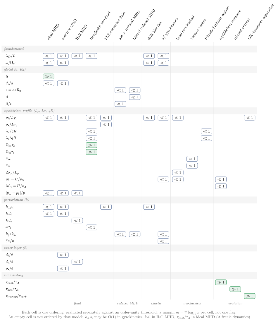
vaft.diagram.ordering_contract_map()Which reduced model assumes which ordering, read from the registered contracts.
vaft.diagram.ordering_contract_map(*, labels=True)Show source vaft/diagram/_orderings.py, lines 335–403
def ordering_contract_map(*, labels: bool = True) -> Diagram:
    r"""Which reduced model assumes which ordering, read from the registered contracts.

    Rows are the ordering quantities of ``vaft.validation.orderings.ORDERING_QUANTITIES``,
    grouped by the scale they are taken on -- foundational, global,
    equilibrium profile, perturbation ($k$), inner layer ($\delta$), time
    history -- so a global $d_i/a$, a mode's $k\,d_i$ and a layer's
    $d_i/\delta$ are separate rows. Columns are the contracts of
    ``CONTRACTS``, grouped by model family; a cell says whether the model
    needs the quantity $\gg 1$ or $\ll 1$, and an empty cell means the model
    does not order it -- $k_\perp\rho_i$ in gyrokinetics, $k\,d_i$ in Hall
    MHD. Every threshold is order unity, and evaluating a state gives a
    continuous margin per cell ($\mp\log_{10}x$), not one valid/invalid flag.
    """
    from vaft.validation.orderings import CONTRACTS, GROUPS, ORDERING_QUANTITIES, SYMBOLS as _SYMBOLS

    labels = _check_labels(labels)
    columns = [name for _, names in _FAMILIES for name in names]
    if sorted(columns) != sorted(CONTRACTS) or set(_SYMBOLS) != set(ORDERING_QUANTITIES):
        raise RuntimeError("ordering_contract_map is out of step with vaft.validation.orderings")
    rows = list(ORDERING_QUANTITIES)
    items: List = []
    right = _LEFT + len(columns) * _COL

    def cx(name):
        return _LEFT + (columns.index(name) + 0.5) * _COL

    for name in columns:
        items.append(Label((cx(name) - 0.15, 0.15), _MODELS[name], "small label,rotate=55", anchor="west",
                           role=f"column:{name}"))
    y = 0.0
    row_y = {}
    for group in GROUPS:
        members = [k for k in rows if ORDERING_QUANTITIES[k].group == group]
        y -= _ROW
        items.append(Polyline.of([(0.0, y - 0.5 * _ROW), (right, y - 0.5 * _ROW), (right, y + 0.5 * _ROW),
                                  (0.0, y + 0.5 * _ROW)], "concept band", role=f"group:{group}", closed=True))
        items.append(Label((0.1, y), _GROUP_TITLES[group], "concept band label", anchor="west",
                           role=f"group:{group}"))
        for key in members:
            y -= _ROW
            row_y[key] = y
            items.append(Label((0.25, y), _SYMBOLS[key], "small label", anchor="west", role=f"row:{key}"))
    bottom = y - 0.5 * _ROW
    for (_, names) in _FAMILIES[1:]:
        x = _LEFT + columns.index(names[0]) * _COL
        items.append(Polyline.of([(x, 0.0), (x, bottom)], "im grid", role="families"))
    for family, names in _FAMILIES:
        x0 = _LEFT + columns.index(names[0]) * _COL
        items.append(Label((x0 + 0.5 * len(names) * _COL, bottom - 0.1), family, "concept band label",
                           anchor="north", role="families"))
    for name in columns:
        for a in CONTRACTS[name].assumptions:
            x, yy = cx(name), row_y[a.quantity]
            text, style = ("$\\gg 1$", "concept source") if a.ordering == "large" else ("$\\ll 1$", "concept leaf")
            items.append(Polyline.of([(x - 0.5, yy - 0.24), (x + 0.5, yy - 0.24), (x + 0.5, yy + 0.24),
                                      (x - 0.5, yy + 0.24)], style, role=f"cell:{name}:{a.quantity}", closed=True))
            items.append(Label((x, yy), text, "small label", role=f"cell:{name}:{a.quantity}"))
    if labels:
        items.append(Label((0.5 * right, bottom - 0.9),
                           "Each cell is one ordering, evaluated separately against an order-unity threshold: "
                           "a margin $m = \\mp\\log_{10}x$ per cell, not one flag.\\\\ "
                           "An empty cell is not ordered by that model: "
                           "$k_\\perp\\rho_i$ may be $O(1)$ in gyrokinetics, $k\\,d_i$ in Hall MHD, "
                           "$\\tau_{evol}/\\tau_A$ in ideal MHD (Alfvenic dynamics)",
                           "note", anchor="north", role="note"))
    model = {"rows": tuple(rows), "columns": tuple(columns),
             "cells": {(n, a.quantity): a.ordering for n in columns for a in CONTRACTS[n].assumptions}}
    return Diagram("ordering_contract_map", Scene(tuple(items)), model=model)
Formats .svg .tex .pdf the SVG above is committed; build the others locally
import vaft.diagram

d = vaft.diagram.ordering_contract_map()
d.tikz  # the TikZ document as text
d.save("ordering_contract_map.svg")  # rendered vector image, the canonical artifact; needs latex, dvisvgm
d.save("ordering_contract_map.tex")  # the complete TikZ document, the text source
d.save("ordering_contract_map.pdf")  # vector PDF; needs pdflatex
adapter_contract_map
1 asset
source
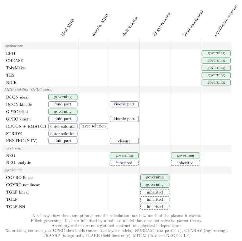
vaft.diagram.adapter_contract_map()Which VAFT code adapter consumes which ordering contract, and in what role.
vaft.diagram.adapter_contract_map(*, labels=True)Show source vaft/diagram/_orderings.py, lines 438–512
def adapter_contract_map(*, labels: bool = True) -> Diagram:
    r"""Which VAFT code adapter consumes which ordering contract, and in what role.

    Rows are the modes of ``vaft.validation.model_contracts.ADAPTER_MODES``,
    grouped by family (equilibrium, MHD stability, neoclassical,
    gyrokinetic); columns are the contracts any of them consumes, in the
    model-family order of :func:`ordering_contract_map`. A cell names how the
    assumption enters the calculation -- not how much of the plasma it covers:
    it *governs* the model solved; it holds for RDCON's ideal *outer solution*
    or its resistive *layer solution*; it underlies DCON-kinetic's *fluid part* or
    drift-kinetic *kinetic part*, or PENTRC's *closure*; or a reduced model
    (TGLF) has *inherited* it from a theory it does not solve. An empty cell
    means no registered contract, not that the calculation is independent of
    that physics. Modes no contract covers are named in the note; the
    validity conditions themselves are documented in the guide, not drawn.
    """
    from vaft.validation.model_contracts import ADAPTER_MODES, ROLES

    labels = _check_labels(labels)
    covered = [m for m in ADAPTER_MODES if m.contracts()[0]]
    uncovered = [m for m in ADAPTER_MODES if not m.contracts()[0]]
    if (set(_ROLE_WORDS) != set(ROLES) or {m.key for m in ADAPTER_MODES} != set(_MODE_NAMES)
            or any(m.family not in _MODE_FAMILIES for m in covered) or {m.key for m in uncovered} != set(_UNCOVERED)):
        raise RuntimeError("adapter_contract_map is out of step with vaft.validation.model_contracts")
    consumed = {u.contract for m in covered for u in m.contracts()[0]}
    columns = [name for _, names in _FAMILIES for name in names if name in consumed]
    right = _ALEFT + len(columns) * _ACOL
    items: List = []

    def cx(name):
        return _ALEFT + (columns.index(name) + 0.5) * _ACOL

    for name in columns:
        items.append(Label((cx(name) - 0.15, 0.15), _MODELS[name], "small label,rotate=55", anchor="west",
                           role=f"column:{name}"))
    y = 0.0
    used = {}
    for family, title in _MODE_FAMILIES.items():
        members = [m for m in covered if m.family == family]
        if not members:
            continue
        y -= _AROW
        items.append(Polyline.of([(0.0, y - 0.5 * _AROW), (right, y - 0.5 * _AROW), (right, y + 0.5 * _AROW),
                                  (0.0, y + 0.5 * _AROW)], "concept band", role=f"family:{family}", closed=True))
        items.append(Label((0.1, y), title, "concept band label", anchor="west", role=f"family:{family}"))
        for mode in members:
            y -= _AROW
            items.append(Label((0.25, y), _MODE_NAMES[mode.key], "small label", anchor="west", role=f"mode:{mode.key}"))
            for use in mode.contracts()[0]:
                x = cx(use.contract)
                used[(mode.key, use.contract)] = use.role
                style = _ROLE_STYLES.get(use.role, "concept leaf")
                items.append(Polyline.of([(x - 1.22, y - 0.24), (x + 1.22, y - 0.24), (x + 1.22, y + 0.24),
                                          (x - 1.22, y + 0.24)], style, role=f"use:{mode.key}:{use.contract}",
                                         closed=True))
                items.append(Label((x, y), _ROLE_WORDS[use.role], "small label",
                                   role=f"use:{mode.key}:{use.contract}"))
    bottom = y - 0.5 * _AROW
    for i in range(1, len(columns)):
        x = _ALEFT + i * _ACOL
        items.append(Polyline.of([(x, 0.0), (x, bottom)], "im grid", role="columns"))
    if labels:
        names = [f"{_MODE_NAMES[m.key]} ({_UNCOVERED[m.key]})" for m in uncovered]
        half = (len(names) + 1) // 2
        none = ", ".join(names[:half]) + ",\\\\ " + ", ".join(names[half:])
        items.append(Label((0.5 * right, bottom - 0.2),
                           "A cell says how the assumption enters the calculation, not how much of the plasma "
                           "it covers.\\\\ Filled: governing. Dashed: inherited by a reduced model that does "
                           "not solve its parent theory.\\\\ An empty cell means no registered contract, "
                           "not physical independence.\\\\ "
                           f"No ordering contract yet: {none}",
                           "note", anchor="north", role="note"))
    model = {"rows": tuple(m.key for m in covered), "columns": tuple(columns), "uses": used,
             "uncovered": tuple(m.key for m in uncovered)}
    return Diagram("adapter_contract_map", Scene(tuple(items)), model=model)
Formats .svg .tex .pdf the SVG above is committed; build the others locally
import vaft.diagram

d = vaft.diagram.adapter_contract_map()
d.tikz  # the TikZ document as text
d.save("adapter_contract_map.svg")  # rendered vector image, the canonical artifact; needs latex, dvisvgm
d.save("adapter_contract_map.tex")  # the complete TikZ document, the text source
d.save("adapter_contract_map.pdf")  # vector PDF; needs pdflatex
Plasma-model guide figures, read from the formalism records (#1739 Phase E2)
Module vaft.diagram._plasma_models
plasma_model_reduction_map
1 asset
source
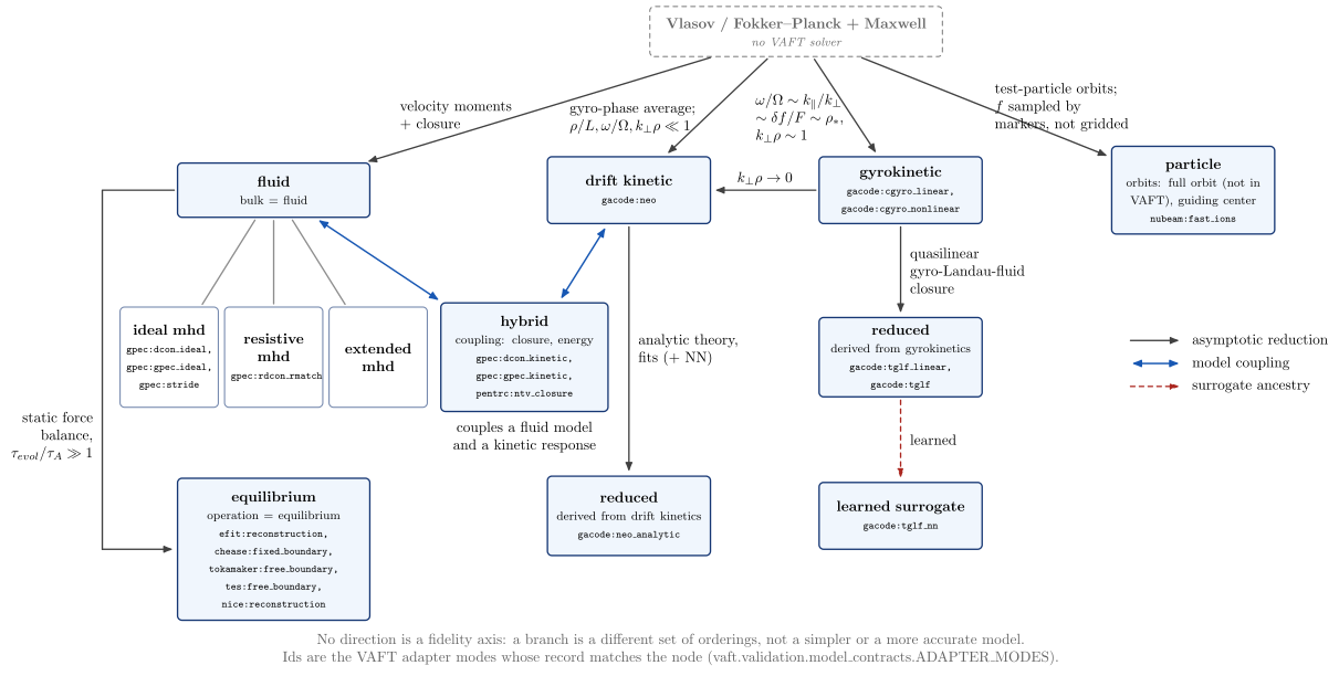
vaft.diagram.plasma_model_reduction_map()One starting point and the reductions to every description VAFT uses.
vaft.diagram.plasma_model_reduction_map(*, labels=True)Formats .svg .tex .pdf the SVG above is committed; build the others locally
import vaft.diagram

d = vaft.diagram.plasma_model_reduction_map()
d.tikz  # the TikZ document as text
d.save("plasma_model_reduction_map.svg")  # rendered vector image, the canonical artifact; needs latex, dvisvgm
d.save("plasma_model_reduction_map.tex")  # the complete TikZ document, the text source
d.save("plasma_model_reduction_map.pdf")  # vector PDF; needs pdflatex
formalism_axes_map
1 asset
source
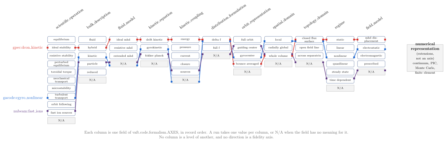
vaft.diagram.formalism_axes_map()The independent axes of a plasma-formalism record, with three runs drawn across them.
vaft.diagram.formalism_axes_map(*, labels=True)Show source vaft/diagram/_plasma_models.py, lines 287–352
def formalism_axes_map(*, labels: bool = True) -> Diagram:
    r"""The independent axes of a plasma-formalism record, with three runs drawn across them.

    One column per field of ``vaft.code.formalism.AXES``, in record order,
    each listing its controlled values and an "N/A" cell (the field has no
    meaning for the run). Three ``ADAPTER_MODES`` runs -- CGYRO nonlinear,
    DCON kinetic, NUBEAM -- are polylines through their values; no column is
    a level of another. The numerical representation is not an axis: it
    stays in ``extensions`` and has its own box, which no run line enters.
    """
    from vaft.code.formalism import AXES
    from vaft.validation.model_contracts import adapter_mode

    labels = _check_labels(labels)
    col, row, top = 2.75, 0.72, 0.0
    width = col - 0.3
    cells: Dict[Tuple[str, str], Tuple[float, float]] = {}
    for j, (field, values) in enumerate(AXES.items()):
        for i, value in enumerate((*values, "N/A")):
            cells[(field, value)] = (j * col, top - (i + 0.5) * row)
    lines: List = []
    marks: List = []
    runs = {}
    for k, (key, colour) in enumerate(_AXES_EXAMPLES):
        record = adapter_mode(key).formalism
        points, dy = [], (k - 1) * 0.14
        for field in AXES:
            value = getattr(record, field)
            x, y = cells[(field, "N/A" if value is None else value)]
            points += [(x - 0.5 * width, y + dy), (x + 0.5 * width, y + dy)]
            for side in (-1, 1):
                marks.append(Polyline.of([(x + side * 0.5 * width - 0.07, y + dy - 0.07),
                                          (x + side * 0.5 * width + 0.07, y + dy - 0.07),
                                          (x + side * 0.5 * width + 0.07, y + dy + 0.07),
                                          (x + side * 0.5 * width - 0.07, y + dy + 0.07)],
                                         f"draw={colour},fill={colour}", role=f"run:{key}", closed=True))
        runs[key] = tuple(getattr(record, f) for f in AXES)
        # the line runs behind the cells: visible between columns, marked at each chosen cell
        lines.append(Polyline.of(points, f"{colour},line width=1.6pt,opacity=0.85", role=f"run:{key}"))
        if labels:
            lines.append(Label((-0.5 * col - 0.15, points[0][1]), escape_latex(key), f"small label,text={colour}",
                               anchor="east", role=f"run:{key}"))
    items: List = list(lines)
    for j, (field, values) in enumerate(AXES.items()):
        x = j * col
        items.append(Label((x - 0.4, top + 0.35), field.replace("_", "\\_"), "small label,rotate=35",
                           anchor="south west", role=f"column:{field}"))
        for value in (*values, "N/A"):
            cx, cy = cells[(field, value)]
            style = _GREY if value == "N/A" else "concept leaf"
            items += list(box(cx, cy, width, row - 0.16, value.replace("_", " "), style=style,
                              text_style="concept text,font=\\scriptsize", role=f"value:{field}:{value}").items)
    items += marks
    depth = max(len(v) for v in AXES.values()) + 1
    bottom = top - depth * row
    side_x = (len(AXES) - 1) * col + 0.5 * col + 2.0
    items += list(box(side_x + 1.4, top - 2.0, 3.2, 2.4, "\\textbf{numerical representation}\\\\ "
                      "{\\footnotesize (extensions, not an axis)}\\\\ {\\footnotesize continuum, PIC, Monte Carlo, "
                      "finite element}", style=_GREY, role="extensions", latex=True).items)
    if labels:
        items.append(Label((0.5 * (len(AXES) - 1) * col, bottom - 0.4),
                           "Each column is one field of vaft.code.formalism.AXES, in record order. A run takes one value "
                           "per column, or N/A when the field has no meaning for it.\\\\ No column is a level of another, "
                           "and no direction is a fidelity axis.", "note", anchor="north", role="note"))
    model = {"columns": tuple(AXES), "runs": runs}
    return Diagram("formalism_axes_map", Scene(tuple(items)), model=model)
Formats .svg .tex .pdf the SVG above is committed; build the others locally
import vaft.diagram

d = vaft.diagram.formalism_axes_map()
d.tikz  # the TikZ document as text
d.save("formalism_axes_map.svg")  # rendered vector image, the canonical artifact; needs latex, dvisvgm
d.save("formalism_axes_map.tex")  # the complete TikZ document, the text source
d.save("formalism_axes_map.pdf")  # vector PDF; needs pdflatex
solver_placement_map
1 asset
source
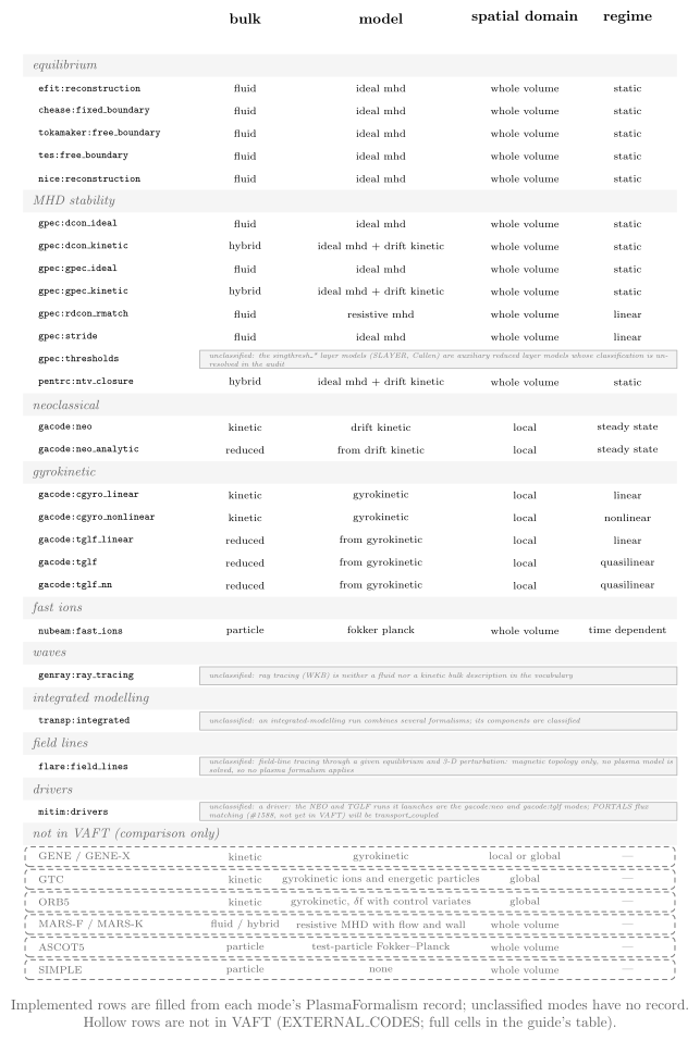
vaft.diagram.solver_placement_map()Every VAFT adapter mode against the main formalism axes, then the codes not in VAFT.
vaft.diagram.solver_placement_map(*, labels=True)Show source vaft/diagram/_plasma_models.py, lines 375–444
def solver_placement_map(*, labels: bool = True) -> Diagram:
    r"""Every VAFT adapter mode against the main formalism axes, then the codes not in VAFT.

    Rows are ``ADAPTER_MODES`` grouped by family; columns the bulk
    description, the fluid model / kinetic equation (or a reduced model's
    parent), the spatial domain and the regime, filled from each record. A
    mode with no record is greyed "unclassified". Below, the codes of
    :data:`EXTERNAL_CODES` are drawn hollow and labelled "not in VAFT", so no
    code looks implemented that is not.
    """
    labels = _check_labels(labels)
    widths = (2.2, 4.4, 2.6, 2.4)
    left, row = 4.3, 0.55
    xs, x = [], left
    for w in widths:
        xs.append(x + 0.5 * w)
        x += w
    right = x
    items: List = []
    for cx, name in zip(xs, _PLACEMENT_COLUMNS):
        items.append(Label((cx, 0.35), name, "small label,font=\\bfseries", anchor="south", role=f"column:{name}"))
    modes = _modes()
    families = [f for f in _FAMILY_ORDER if any(m.family == f for m in modes)]
    families += sorted({m.family for m in modes} - set(families))
    y = 0.0
    placed = {}
    for family in families:
        y -= row
        items.append(Polyline.of([(0.0, y - 0.5 * row), (right, y - 0.5 * row), (right, y + 0.5 * row),
                                  (0.0, y + 0.5 * row)], "concept band", role=f"family:{family}", closed=True))
        items.append(Label((0.1, y), escape_latex(_FAMILY_TITLES.get(family, family)), "concept band label", anchor="west",
                           role=f"family:{family}"))
        for mode in (m for m in modes if m.family == family):
            y -= row
            items.append(Label((0.25, y), escape_latex(mode.key), "small label,font=\\ttfamily\\scriptsize",
                               anchor="west", role=f"mode:{mode.key}"))
            if mode.formalism is None:
                items.append(Polyline.of([(left, y - 0.22), (right, y - 0.22), (right, y + 0.22), (left, y + 0.22)],
                                         _GREY, role=f"mode:{mode.key}", closed=True))
                items.append(Label((left + 0.1, y), "unclassified: " + _tex(mode.note),
                                   f"small label,text=black!55,font=\\itshape\\tiny,text width={right - left - 0.3:.2f}cm,"
                                   "align=left", anchor="west", role=f"mode:{mode.key}"))
                placed[mode.key] = None
                continue
            r = mode.formalism
            values = (r.bulk_description, _model_cell(r), r.spatial_domain or "—", r.regime or "—")
            placed[mode.key] = values
            for cx, w, v in zip(xs, widths, values):
                items.append(Label((cx, y), _tex(v).replace("\\_", " "), "small label,font=\\scriptsize",
                                   role=f"cell:{mode.key}"))
    y -= row
    items.append(Polyline.of([(0.0, y - 0.5 * row), (right, y - 0.5 * row), (right, y + 0.5 * row),
                              (0.0, y + 0.5 * row)], "concept band", role="family:external", closed=True))
    items.append(Label((0.1, y), "not in VAFT (comparison only)", "concept band label", anchor="west",
                       role="family:external"))
    for code in EXTERNAL_CODES:
        y -= row
        items.append(Polyline.of([(0.05, y - 0.24), (right - 0.05, y - 0.24), (right - 0.05, y + 0.24),
                                  (0.05, y + 0.24)], _HOLLOW, role=f"external:{code.code}", closed=True))
        items.append(Label((0.25, y), _tex(code.code), "small label,text=black!60,font=\\scriptsize",
                           anchor="west", role=f"external:{code.code}"))
        for cx, v in zip(xs, (code.bulk, code.model.split(";")[0].split(" (")[0], code.domain.split(";")[0], "—")):
            items.append(Label((cx, y), _tex(v), "small label,text=black!60,font=\\scriptsize",
                               role=f"external:{code.code}"))
    if labels:
        items.append(Label((0.5 * right, y - 0.6), "Implemented rows are filled from each mode's PlasmaFormalism record; "
                           "unclassified modes have no record.\\\\ Hollow rows are not in VAFT "
                           "(EXTERNAL\\_CODES; full cells in the guide's table).", "note", anchor="north", role="note"))
    model = {"rows": placed, "external": tuple(c.code for c in EXTERNAL_CODES), "families": tuple(families)}
    return Diagram("solver_placement_map", Scene(tuple(items)), model=model)
Formats .svg .tex .pdf the SVG above is committed; build the others locally
import vaft.diagram

d = vaft.diagram.solver_placement_map()
d.tikz  # the TikZ document as text
d.save("solver_placement_map.svg")  # rendered vector image, the canonical artifact; needs latex, dvisvgm
d.save("solver_placement_map.tex")  # the complete TikZ document, the text source
d.save("solver_placement_map.pdf")  # vector PDF; needs pdflatex
kinetic_mhd_coupling
1 asset
source
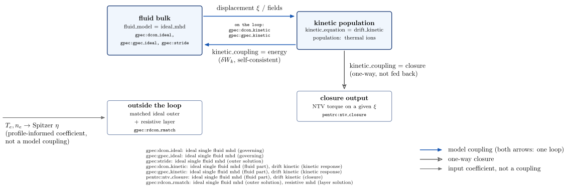
vaft.diagram.kinetic_mhd_coupling()Kinetic-MHD as a loop between a fluid bulk and a drift-kinetic population.
vaft.diagram.kinetic_mhd_coupling(*, labels=True)Formats .svg .tex .pdf the SVG above is committed; build the others locally
import vaft.diagram

d = vaft.diagram.kinetic_mhd_coupling()
d.tikz  # the TikZ document as text
d.save("kinetic_mhd_coupling.svg")  # rendered vector image, the canonical artifact; needs latex, dvisvgm
d.save("kinetic_mhd_coupling.tex")  # the complete TikZ document, the text source
d.save("kinetic_mhd_coupling.pdf")  # vector PDF; needs pdflatex
reduced_model_ancestry
1 asset
source
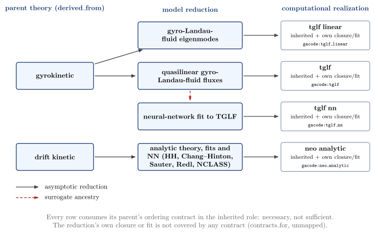
vaft.diagram.reduced_model_ancestry()Parent theory, model reduction and computational realization of every reduced mode.
vaft.diagram.reduced_model_ancestry(*, labels=True)Show source vaft/diagram/_plasma_models.py, lines 558–609
def reduced_model_ancestry(*, labels: bool = True) -> Diagram:
    r"""Parent theory, model reduction and computational realization of every reduced mode.

    Rows are the ``ADAPTER_MODES`` with ``bulk_description="reduced"``;
    the left column is their ``derived_from`` theory, the middle the
    reduction, the right the VAFT mode that realizes it. Parent to reduction
    is an asymptotic reduction; TGLF to TGLF-NN a surrogate's ancestry. Every
    row consumes its parent's contract in the ``inherited`` role, and adds a
    closure or fit no ordering contract covers.
    """
    from vaft.validation.model_contracts import ADAPTER_MODES

    labels = _check_labels(labels)
    reduced = [m for m in ADAPTER_MODES if m.formalism is not None and m.formalism.bulk_description == "reduced"]
    if {m.key for m in reduced} != set(_REDUCTIONS):
        raise RuntimeError("reduced_model_ancestry is out of step with ADAPTER_MODES")
    items: List = []
    xs, row = (-7.0, 0.0, 7.0), 2.1
    for x, title in zip(xs, ("parent theory (derived\\_from)", "model reduction", "computational realization")):
        items.append(Label((x, 1.1), title, "concept group title", anchor="south", role="column"))
    parents: Dict[str, Box] = {}
    reductions: Dict[str, Box] = {}
    # parents grouped; within a parent, models before their surrogates, in registry order
    order = sorted(reduced, key=lambda m: (m.formalism.derived_from != "gyrokinetic", m.key in _SURROGATES))
    for i, mode in enumerate(order):
        y = -i * row
        parent = mode.formalism.derived_from
        reduction = _node(xs[1], y, 5.4, 1.4, _REDUCTIONS[mode.key], (), role=f"reduction:{mode.key}")
        realization = _node(xs[2], y, 4.6, 1.5, mode.key.split(":")[1].replace("_", " "), [mode.key],
                            detail="inherited + own closure/fit", style="concept leaf", role=f"mode:{mode.key}")
        reductions[mode.key] = reduction
        items += list(reduction.items) + list(realization.items)
        items.append(connector(reduction, realization, style="connector", role="edge:realization"))
        if parent not in parents:
            members = [m for m in order if m.formalism.derived_from == parent]
            first, last = order.index(members[0]), order.index(members[-1])
            parents[parent] = _node(xs[0], -0.5 * (first + last) * row, 4.0, 1.4, parent.replace("_", " "), (),
                                    role=f"parent:{parent}")
            items += list(parents[parent].items)
        if mode.key not in _SURROGATES:
            # a surrogate descends from TGLF (dashed, below), not by reduction from the theory
            items.append(_edge(parents[parent], reduction, "asymptotic_reduction"))
    for surrogate, model in _SURROGATES.items():
        items.append(_edge(reductions[model], reductions[surrogate], "surrogate_ancestry"))
    bottom = -(len(order) - 0.4) * row
    if labels:
        items += _legend(("asymptotic_reduction", "surrogate_ancestry"), xs[0] - 2.0, bottom - 0.3)
        items.append(Label((xs[1], bottom - 1.6), "Every row consumes its parent's ordering contract in the inherited "
                           "role: necessary, not sufficient.\\\\ The reduction's own closure or fit is not covered by "
                           "any contract (contracts\\_for, unmapped).", "note", anchor="north", role="note"))
    model = {"rows": tuple(m.key for m in order), "parents": {m.key: m.formalism.derived_from for m in order}}
    return Diagram("reduced_model_ancestry", Scene(tuple(items)), model=model)
Formats .svg .tex .pdf the SVG above is committed; build the others locally
import vaft.diagram

d = vaft.diagram.reduced_model_ancestry()
d.tikz  # the TikZ document as text
d.save("reduced_model_ancestry.svg")  # rendered vector image, the canonical artifact; needs latex, dvisvgm
d.save("reduced_model_ancestry.tex")  # the complete TikZ document, the text source
d.save("reduced_model_ancestry.pdf")  # vector PDF; needs pdflatex
Tokamak toroidal geometry and flux coordinates
Module vaft.diagram._tokamak_geometry
tokamak_torus
2 assets
source
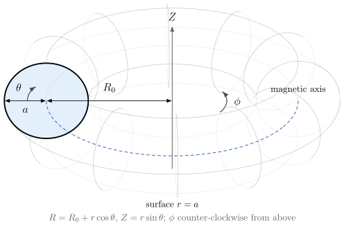
vaft.diagram.tokamak_torus(projection='3d')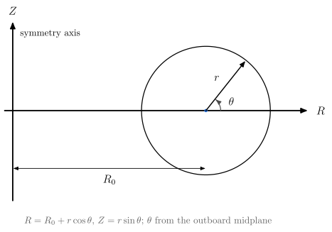
vaft.diagram.tokamak_torus(projection='poloidal')The tokamak torus: major radius $R_0$, minor radius $a$, toroidal $\phi$ and poloidal $\theta$.
vaft.diagram.tokamak_torus(projection='3d', *, labels=True)Formats .svg .tex .pdf the SVG above is committed; build the others locally
import vaft.diagram

d = vaft.diagram.tokamak_torus(projection='3d')
d.tikz  # the TikZ document as text
d.save("tokamak_torus_3d.svg")  # rendered vector image, the canonical artifact; needs latex, dvisvgm
d.save("tokamak_torus_3d.tex")  # the complete TikZ document, the text source
d.save("tokamak_torus_3d.pdf")  # vector PDF; needs pdflatex
Formula functions referenced:
equilibrium.miller_surface
flux_surfaces
2 assets
source
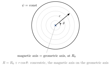
vaft.diagram.flux_surfaces(shape='circular')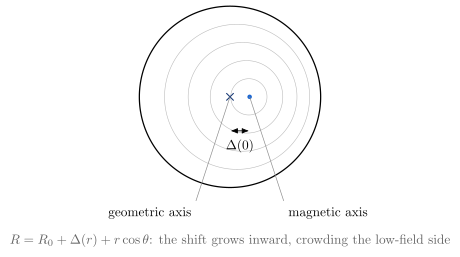
vaft.diagram.flux_surfaces(shape='shifted')Nested circular flux surfaces, concentric or Shafranov-shifted.
vaft.diagram.flux_surfaces(shape='circular', *, labels=True)Show source vaft/diagram/_tokamak_geometry.py, lines 219–282
def flux_surfaces(shape: str = "circular", *, labels: bool = True) -> Diagram:
    r"""Nested circular flux surfaces, concentric or Shafranov-shifted.

    ``"circular"``: $R = R_0 + r\cos\theta$, $Z = r\sin\theta$, the magnetic
    axis on the geometric axis. ``"shifted"``: each surface's centre moves
    out by ``shafranov_shift_from_r_a_R0_beta_p_li`` (schematic
    $\beta_p = 0.8$, $l_i = 1$), zero at the boundary and largest on the
    magnetic axis, which now sits outside the geometric axis.
    """
    if shape not in _SHAPES:
        raise ValueError(f"shape must be one of {_SHAPES}, not {shape!r}")
    labels = _check_labels(labels)
    radii = _A * np.array([0.2, 0.4, 0.6, 0.8, 1.0])
    shifts = (shafranov_shift_from_r_a_R0_beta_p_li(radii, _A, _R0, _BETA_P, _L_I) if shape == "shifted"
              else np.zeros_like(radii))
    axis_shift = (shafranov_shift_from_r_a_R0_beta_p_li(0.0, _A, _R0, _BETA_P, _L_I) if shape == "shifted" else 0.0)
    items: List = []
    for r, d in zip(radii, shifts):
        items.append(Polyline.of(_surface(r, shift=d), "lcfs" if r == _A else "surface", role="flux_surface",
                                 closed=True))
    geometric = (0.0, 0.0)
    magnetic = (axis_shift * _CM, 0.0)
    items += [Marker(magnetic, "o", "opoint", role="magnetic_axis"),
              Marker(geometric, "x", "xpoint", role="geometric_axis")]
    if labels:
        top = _A * _CM
        if shape == "shifted":
            below = -top - 0.35
            items += [
                Polyline.of([magnetic, (magnetic[0] + 0.9, below)], "leader line", role="magnetic_axis"),
                Label((magnetic[0] + 0.9, below - 0.05), "magnetic axis", "small label", anchor="north west",
                      role="magnetic_axis"),
                Polyline.of([geometric, (geometric[0] - 0.9, below)], "leader line", role="geometric_axis"),
                Label((geometric[0] - 0.9, below - 0.05), "geometric axis", "small label", anchor="north east",
                      role="geometric_axis"),
            ]
        else:
            th = 0.7
            tip = (0.8 * _A * _CM * math.cos(th), 0.8 * _A * _CM * math.sin(th))
            items += [
                Polyline.of([(0.0, 0.0), (-0.9, -top - 0.35)], "leader line", role="magnetic_axis"),
                Label((-0.9, -top - 0.4), "magnetic axis $=$ geometric axis, at $R_0$", "small label",
                      anchor="north", role="magnetic_axis"),
                Arrow((0.0, 0.0), tip, "vector", role="minor_radius"),
                Label((0.5 * tip[0] - 0.1, 0.5 * tip[1] + 0.1), "$r$", "small label", anchor="south east",
                      role="minor_radius"),
                Polyline.of(np.stack([0.5 * np.cos(np.linspace(0, th, 20)), 0.5 * np.sin(np.linspace(0, th, 20))], -1),
                            "angle arc", role="poloidal_angle"),
                Label((0.65 * math.cos(th / 2), 0.65 * math.sin(th / 2)), "$\\theta$", "small label",
                      anchor="west", role="poloidal_angle"),
                Label((-0.72 * _A * _CM, 0.72 * _A * _CM), "$\\psi = $ const", "small label", anchor="south east",
                      role="flux_surface"),
            ]
        if shape == "shifted":
            items += [Arrow((0.0, -0.9), (magnetic[0], -0.9), "width arrow", role="shift", both=True),
                      Label((0.5 * magnetic[0], -1.0), "$\\Delta(0)$", "small label", anchor="north", role="shift"),
                      _note("$R = R_0 + \\Delta(r) + r\\cos\\theta$: the shift grows inward, crowding the low-field side",
                            0.0, -top - 1.1)]
        else:
            items.append(_note("$R = R_0 + r\\cos\\theta$: concentric, the magnetic axis on the geometric axis",
                               0.0, -top - 1.1))
    model = {"shape": shape, "radii": radii, "shifts": shifts, "axis_shift": axis_shift,
             "R0": _R0, "a": _A, "beta_p": _BETA_P, "l_i": _L_I}
    return Diagram(f"flux_surfaces_{shape}", Scene(tuple(items)), model=model)
Formats .svg .tex .pdf the SVG above is committed; build the others locally
import vaft.diagram

d = vaft.diagram.flux_surfaces(shape='circular')
d.tikz  # the TikZ document as text
d.save("flux_surfaces_circular.svg")  # rendered vector image, the canonical artifact; needs latex, dvisvgm
d.save("flux_surfaces_circular.tex")  # the complete TikZ document, the text source
d.save("flux_surfaces_circular.pdf")  # vector PDF; needs pdflatex
Formula functions referenced:
equilibrium.miller_surface, equilibrium.shafranov_shift_from_r_a_R0_beta_p_li
shaping_family
1 asset
source
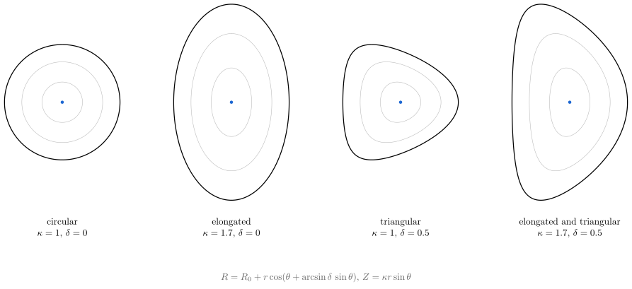
vaft.diagram.shaping_family()Elongation $\kappa$ and triangularity $\delta$ on one boundary family.
vaft.diagram.shaping_family(*, labels=True)Show source vaft/diagram/_tokamak_geometry.py, lines 293–320
def shaping_family(*, labels: bool = True) -> Diagram:
    r"""Elongation $\kappa$ and triangularity $\delta$ on one boundary family.

    Four cross-sections from ``miller_surface``: circular, $\kappa = 1.7$,
    $\delta = 0.5$, and both, each with nested surfaces at
    $\delta(r) = \delta\,r/a$ and constant $\kappa$. The top of a surface
    sits at $R_0 - \delta r$: positive triangularity makes the D.
    """
    labels = _check_labels(labels)
    items: List = []
    gap = 2.9 * _A * _CM / 1.1
    boundaries = {}
    for i, (name, kappa, delta) in enumerate(_FAMILY):
        x0 = i * gap
        for r in _A * np.array([0.35, 0.7, 1.0]):
            pts = _surface(r, kappa, delta * r / _A) * 0.9 + np.array([x0, 0.0])
            items.append(Polyline.of(pts, "lcfs" if r == _A else "surface", role=f"shape:{name}", closed=True))
            if r == _A:
                boundaries[name] = pts
        items.append(Marker((x0, 0.0), "o", "opoint", role=f"shape:{name}"))
        if labels:
            items.append(Label((x0, -1.95 * _A * _CM * 0.9), f"{name}\\\\ $\\kappa = {kappa:g}$, $\\delta = {delta:g}$",
                               "small label,align=center", anchor="north", role=f"shape:{name}"))
    if labels:
        items.append(_note("$R = R_0 + r\\cos(\\theta + \\arcsin\\delta\\,\\sin\\theta)$, $Z = \\kappa r\\sin\\theta$",
                           1.5 * gap, -2.9 * _A * _CM * 0.9))
    model = {"family": _FAMILY, "boundaries": boundaries}
    return Diagram("shaping_family", Scene(tuple(items)), model=model)
Formats .svg .tex .pdf the SVG above is committed; build the others locally
import vaft.diagram

d = vaft.diagram.shaping_family()
d.tikz  # the TikZ document as text
d.save("shaping_family.svg")  # rendered vector image, the canonical artifact; needs latex, dvisvgm
d.save("shaping_family.tex")  # the complete TikZ document, the text source
d.save("shaping_family.pdf")  # vector PDF; needs pdflatex
Formula functions referenced:
equilibrium.miller_surface
hfs_lfs_field
1 asset
source
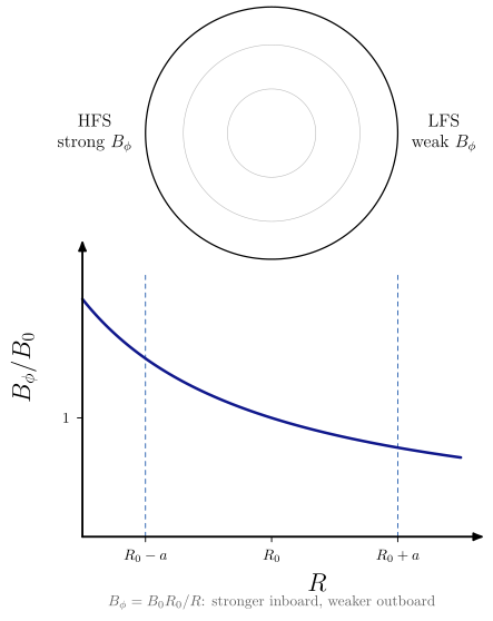
vaft.diagram.hfs_lfs_field()$B_\phi \propto 1/R$: the high-field side is inboard, the low-field side outboard.
vaft.diagram.hfs_lfs_field(*, labels=True)Show source vaft/diagram/_tokamak_geometry.py, lines 328–372
def hfs_lfs_field(*, labels: bool = True) -> Diagram:
    r"""$B_\phi \propto 1/R$: the high-field side is inboard, the low-field side outboard.

    The cross-section above shares its $R$ axis with $B_\phi(R)$ from
    ``vacuum_toroidal_field`` below: across the plasma the field falls from
    $B_0R_0/(R_0 - a)$ inboard to $B_0R_0/(R_0 + a)$ outboard.
    """
    labels = _check_labels(labels)
    B0 = 1.0
    R = np.linspace(_R0 - 1.5 * _A, _R0 + 1.5 * _A, 201)
    B = vacuum_toroidal_field(B0, _R0, R)
    chart = Chart(x_range=(float(R[0]), float(R[-1])), y_range=(0.0, 1.15 * float(B.max())))
    chart.curves["B_phi"] = np.stack([R, B], axis=-1)
    chart.curves["plasma_in"] = np.array([[_R0 - _A, 0.0], [_R0 - _A, 1.1 * B.max()]])
    chart.curves["plasma_out"] = np.array([[_R0 + _A, 0.0], [_R0 + _A, 1.1 * B.max()]])
    chart.parameters.update({"B_hfs": float(vacuum_toroidal_field(B0, _R0, _R0 - _A)),
                             "B_lfs": float(vacuum_toroidal_field(B0, _R0, _R0 + _A)), "B0": B0})
    ticks = (_R0 - _A, _R0, _R0 + _A)
    scene = render_chart(
        chart, x_label="$R$", y_label="$B_\\phi/B_0$",
        curve_styles={"plasma_in": "rational", "plasma_out": "rational", "B_phi": "boundary"},
        region_text={}, x_ticks=ticks, x_tick_text=("$R_0 - a$", "$R_0$", "$R_0 + a$"),
        y_ticks=(1.0,), y_tick_text=("$1$",),
    )
    # the cross-section, on the chart's R scale, above it
    to_cm = lambda RR, ZZ: np.stack([chart.to_cm(np.stack([RR, 0 * RR], -1))[..., 0],  # noqa: E731
                                     np.asarray(ZZ) * CHART_WIDTH / (R[-1] - R[0]) + 9.6], axis=-1)
    theta = np.linspace(0.0, 2.0 * math.pi, 241)
    Rb, Zb = miller_surface(_A, theta, _R0, 1.0, 0.0)
    items: List = [Polyline.of(to_cm(Rb, Zb), "lcfs", role="boundary", closed=True)]
    for r in (0.35, 0.7):
        Rs, Zs = miller_surface(r * _A, theta, _R0, 1.0, 0.0)
        items.append(Polyline.of(to_cm(Rs, Zs), "surface", role="flux_surface", closed=True))
    if labels:
        hfs = to_cm(np.array([_R0 - _A]), np.array([0.0]))[0]
        lfs = to_cm(np.array([_R0 + _A]), np.array([0.0]))[0]
        items += [
            Label((float(hfs[0]) - 0.2, float(hfs[1])), "HFS\\\\ strong $B_\\phi$", "label,align=center",
                  anchor="east", role="hfs"),
            Label((float(lfs[0]) + 0.2, float(lfs[1])), "LFS\\\\ weak $B_\\phi$", "label,align=center",
                  anchor="west", role="lfs"),
            Label((CHART_WIDTH / 2, -1.25), "$B_\\phi = B_0R_0/R$: stronger inboard, weaker outboard", "note",
                  anchor="north", role="note"),
        ]
    return Diagram("hfs_lfs_field", scene + Scene(tuple(items)), model=chart)
Formats .svg .tex .pdf the SVG above is committed; build the others locally
import vaft.diagram

d = vaft.diagram.hfs_lfs_field()
d.tikz  # the TikZ document as text
d.save("hfs_lfs_field.svg")  # rendered vector image, the canonical artifact; needs latex, dvisvgm
d.save("hfs_lfs_field.tex")  # the complete TikZ document, the text source
d.save("hfs_lfs_field.pdf")  # vector PDF; needs pdflatex
Formula functions referenced:
equilibrium.miller_surface, equilibrium.vacuum_toroidal_field
safety_factor_winding
1 asset
source
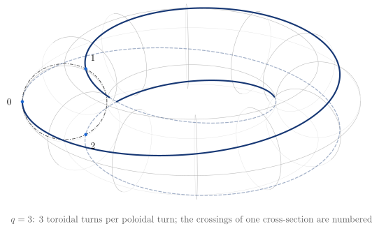
vaft.diagram.safety_factor_winding()$q$ is the number of toroidal turns a field line makes per poloidal turn.
vaft.diagram.safety_factor_winding(q=3, *, labels=True)Show source vaft/diagram/_tokamak_geometry.py, lines 380–415
def safety_factor_winding(q: int = 3, *, labels: bool = True) -> Diagram:
    r"""$q$ is the number of toroidal turns a field line makes per poloidal turn.

    A straight field line $\theta = \phi/q$ on a circular surface, followed
    for one poloidal transit, crosses a cross-section facing the camera $q$ times; the
    crossings are numbered in order. $q$ is a positive integer from 1 to 5 here.
    """
    if isinstance(q, bool) or not isinstance(q, (int, np.integer)) or not 1 <= q <= 5:
        raise ValueError(f"q must be an integer from 1 to 5, not {q!r}")
    labels = _check_labels(labels)
    phi_cut = _camera_cut()
    items: List = _torus_wireframe()
    t = np.linspace(0.0, 2.0 * math.pi, 121)
    items.append(Polyline.of(_p3(_torus(_A, t, np.full_like(t, phi_cut))), "cut", role="cross_section",
                             closed=True))
    phi = np.linspace(phi_cut, phi_cut + 2.0 * math.pi * q, 1200 * q + 1)
    theta = (phi - phi_cut) / q
    line = _torus(_A, theta, phi)
    items += split(_p3(line), _visible(_torus_normal(theta, phi), line), "field line", "field line hidden",
                   "field_line")
    crossings = []
    for k in range(q + 1):
        point = _torus(_A, 2.0 * math.pi * k / q, phi_cut)
        crossings.append(point)
        if k < q:
            items.append(Marker(tuple(_p3(point)), "o", "opoint", role="crossing"))
            if labels:
                outward = _p3(point) - _p3(np.array([_R0 * math.cos(phi_cut), _R0 * math.sin(phi_cut), 0.0]))
                outward = outward / (np.linalg.norm(outward) or 1.0)
                items.append(Label(tuple(_p3(point) + 0.5 * outward), f"${k}$" if k else "$0$",
                                   "small label", anchor="center", role="crossing"))
    if labels:
        items.append(_note(f"$q = {q}$: {q} toroidal turn{'s' if q > 1 else ''} per poloidal turn; "
                           "the crossings of one cross-section are numbered", float(_p3(np.zeros(3))[0]), _below(items)))
    model = {"q": q, "field_line": line, "crossings": np.array(crossings), "phi_cut": phi_cut}
    return Diagram("safety_factor_winding", Scene(tuple(items)), model=model)
Formats .svg .tex .pdf the SVG above is committed; build the others locally
import vaft.diagram

d = vaft.diagram.safety_factor_winding()
d.tikz  # the TikZ document as text
d.save("safety_factor_winding.svg")  # rendered vector image, the canonical artifact; needs latex, dvisvgm
d.save("safety_factor_winding.tex")  # the complete TikZ document, the text source
d.save("safety_factor_winding.pdf")  # vector PDF; needs pdflatex
flux_coordinates
1 asset
source
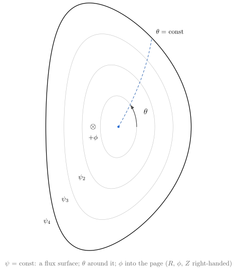
vaft.diagram.flux_coordinates()Flux coordinates $(\psi, \theta, \phi)$ on a shaped cross-section.
vaft.diagram.flux_coordinates(*, labels=True)Show source vaft/diagram/_tokamak_geometry.py, lines 433–470
def flux_coordinates(*, labels: bool = True) -> Diagram:
    r"""Flux coordinates $(\psi, \theta, \phi)$ on a shaped cross-section.

    $\psi$ labels the nested surfaces, $\theta$ runs around each from the
    outboard midplane, and $\phi$ is the ignorable toroidal angle: with $R$
    to the right and $Z$ up, $+\phi$ points into the page. A coordinate line
    of constant $\theta$ crosses every surface.
    """
    labels = _check_labels(labels)
    model = _shaped_model()
    scale = _CM * 1.6
    items: List = []
    radii = np.array([0.25, 0.5, 0.75, 1.0])
    theta = np.linspace(0.0, 2.0 * math.pi, 241)
    for r in radii:
        pts = model.section(r, theta) * scale
        items.append(Polyline.of(pts, "lcfs" if r == 1.0 else "surface", role="flux_surface", closed=True))
    th0 = 0.8
    line = np.array([model.section(r, th0) for r in np.linspace(0.0, 1.0, 41)]) * scale
    items += [Polyline.of(line, "rational", role="theta_line"), Marker((0.0, 0.0), "o", "opoint", role="magnetic_axis"),
              Label((-0.35 * scale, 0.0), "$\\otimes$", "label", anchor="center", role="toroidal_angle")]
    arc = np.array([model.section(0.25, t) for t in np.linspace(0.0, th0, 20)]) * scale
    items.append(Polyline.of(arc, "angle arc", role="poloidal_angle"))
    if labels:
        for r in radii[1:]:
            p = model.section(r, math.pi * 1.25) * scale
            items.append(Label(tuple(p + np.array([-0.08, -0.08])), f"$\\psi_{{{int(r * 4)}}}$", "small label",
                               anchor="north east", role="flux_surface"))
        mid = model.section(0.32, th0 / 2) * scale
        items += [
            Label(tuple(mid + np.array([0.1, 0.0])), "$\\theta$", "label", anchor="west", role="poloidal_angle"),
            Label(tuple(line[-1] + np.array([0.1, 0.1])), "$\\theta = $ const", "small label", anchor="south west",
                  role="theta_line"),
            Label((-0.35 * scale, -0.3), "$+\\phi$", "small label", anchor="north", role="toroidal_angle"),
            _note("$\\psi$ = const: a flux surface; $\\theta$ around it; $\\phi$ into the page ($R$, $\\phi$, $Z$ right-handed)",
                  0.0, -_KAPPA * scale - 0.4),
        ]
    return Diagram("flux_coordinates", Scene(tuple(items)), model={"radii": radii, "theta_line": th0})
Formats .svg .tex .pdf the SVG above is committed; build the others locally
import vaft.diagram

d = vaft.diagram.flux_coordinates()
d.tikz  # the TikZ document as text
d.save("flux_coordinates.svg")  # rendered vector image, the canonical artifact; needs latex, dvisvgm
d.save("flux_coordinates.tex")  # the complete TikZ document, the text source
d.save("flux_coordinates.pdf")  # vector PDF; needs pdflatex
poloidal_angle_comparison
1 asset
source
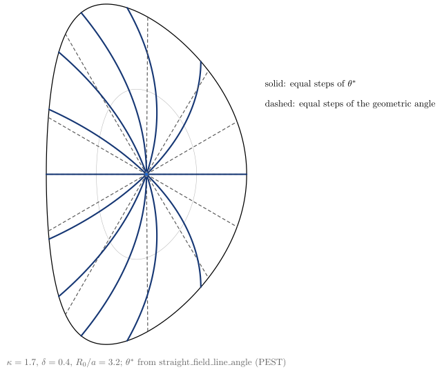
vaft.diagram.poloidal_angle_comparison()The geometric poloidal angle and the straight-field-line angle $\theta^*$ are different coordinates.
vaft.diagram.poloidal_angle_comparison(*, labels=True)Show source vaft/diagram/_tokamak_geometry.py, lines 473–513
def poloidal_angle_comparison(*, labels: bool = True) -> Diagram:
    r"""The geometric poloidal angle and the straight-field-line angle $\theta^*$ are different coordinates.

    On the shaped surfaces, dashed rays are equal steps of the geometric
    angle measured from the magnetic axis; solid curves are equal steps of
    the PEST $\theta^*$ of ``straight_field_line_angle``, along which a field
    line advances uniformly. They coincide only on circular surfaces at
    infinite aspect ratio; here $\theta^*$ lines crowd towards the inboard side.
    """
    labels = _check_labels(labels)
    model = _shaped_model()
    scale = _CM * 1.6
    items: List = []
    theta = np.linspace(0.0, 2.0 * math.pi, 241)
    for r in (0.5, 1.0):
        items.append(Polyline.of(model.section(r, theta) * scale, "lcfs" if r == 1.0 else "surface",
                                 role="flux_surface", closed=True))
    r_grid = np.linspace(0.02, 1.0, 50)
    star_lines = {}
    for k in range(12):
        target = 2.0 * math.pi * k / 12
        # geometric ray: straight from the axis to where the boundary has this polar angle
        boundary = model.section(1.0, theta)
        polar = np.mod(np.arctan2(boundary[:, 1], boundary[:, 0]), 2.0 * math.pi)
        j = int(np.argmin(np.abs(np.angle(np.exp(1j * (polar - target))))))
        items.append(Polyline.of([(0.0, 0.0), tuple(boundary[j] * scale)], "approx", role="geometric_angle"))
        pts = np.array([model.section(r, model.theta_from_star(r, target)) for r in r_grid])
        star_lines[k] = pts
        items.append(Polyline.of(pts * scale, "field line", role="straight_field_line_angle"))
    items.append(Marker((0.0, 0.0), "o", "opoint", role="magnetic_axis"))
    if labels:
        items += [
            Label((1.15 * scale, 0.9 * scale), "solid: equal steps of $\\theta^*$", "small label", anchor="west",
                  role="straight_field_line_angle"),
            Label((1.15 * scale, 0.7 * scale), "dashed: equal steps of the geometric angle", "small label",
                  anchor="west", role="geometric_angle"),
            _note(f"$\\kappa = {_KAPPA:g}$, $\\delta = {_DELTA:g}$, $R_0/a = {_ASPECT:g}$; "
                  "$\\theta^*$ from straight\\_field\\_line\\_angle (PEST)", 0.0, -_KAPPA * scale - 0.4),
        ]
    return Diagram("poloidal_angle_comparison", Scene(tuple(items)),
                   model={"theta_star_lines": star_lines, "island_model": model})
Formats .svg .tex .pdf the SVG above is committed; build the others locally
import vaft.diagram

d = vaft.diagram.poloidal_angle_comparison()
d.tikz  # the TikZ document as text
d.save("poloidal_angle_comparison.svg")  # rendered vector image, the canonical artifact; needs latex, dvisvgm
d.save("poloidal_angle_comparison.tex")  # the complete TikZ document, the text source
d.save("poloidal_angle_comparison.pdf")  # vector PDF; needs pdflatex
unwrapped_flux_surface
1 asset
source
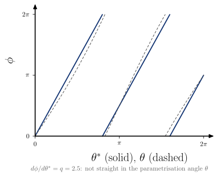
vaft.diagram.unwrapped_flux_surface()On an unwrapped flux surface a field line is straight in $(\theta^, \phi)$: $d\phi/d\theta^ = q$.
vaft.diagram.unwrapped_flux_surface(q=2.5, *, labels=True)Show source vaft/diagram/_tokamak_geometry.py, lines 516–561
def unwrapped_flux_surface(q: float = 2.5, *, labels: bool = True) -> Diagram:
    r"""On an unwrapped flux surface a field line is straight in $(\theta^*, \phi)$: $d\phi/d\theta^* = q$.

    The solid lines are one field line of safety factor $q$ in
    straight-field-line coordinates, wrapped at $\phi = 2\pi$. The dashed
    curve is the same field line against the shaped surface's
    parametrisation angle $\theta$ (the $r = 0.55$ surface of the reference
    D shape): straight in a straight-field-line angle, not in $\theta$.
    """
    try:
        q = float(q)
    except (TypeError, ValueError):
        raise ValueError(f"q must be a number, not {q!r}") from None
    if not (math.isfinite(q) and 0.5 <= q <= 6.0):
        raise ValueError(f"q must lie in [0.5, 6] for a readable figure, not {q!r}")
    labels = _check_labels(labels)
    model = _shaped_model()
    two_pi = 2.0 * math.pi
    chart = Chart(x_range=(0.0, two_pi), y_range=(0.0, two_pi))
    theta_star = np.linspace(0.0, two_pi, 1201)
    phi = q * theta_star
    wraps = np.floor(phi / two_pi).astype(int)
    theta_geo = model.theta_from_star(0.55, theta_star)
    for k in np.unique(wraps):
        sel = wraps == k
        if sel.sum() < 2:
            continue
        chart.curves[f"straight_{k}"] = np.stack([theta_star[sel], phi[sel] - two_pi * k], axis=-1)
        # the same points against the parametrisation angle
        chart.curves[f"parametrisation_{k}"] = np.stack([theta_geo[sel], phi[sel] - two_pi * k], axis=-1)
    chart.parameters.update({"q": q})
    ticks = (0.0, math.pi, two_pi)
    tick_text = ("$0$", "$\\pi$", "$2\\pi$")
    styles = {name: ("field line" if name.startswith("straight") else "approx") for name in chart.curves}
    scene = render_chart(chart, x_label="$\\theta^*$ (solid), $\\theta$ (dashed)", y_label="$\\phi$",
                         curve_styles=styles, region_text={}, x_ticks=ticks, y_ticks=ticks,
                         x_tick_text=tick_text, y_tick_text=tick_text)
    items = [Polyline(it.points, it.style,
                      "field_line" if it.role.startswith("straight") else "parametrisation_angle", it.closed)
             if isinstance(it, Polyline) and it.role.startswith(("straight", "parametrisation")) else it
             for it in scene.items]
    if labels:
        items.append(Label((CHART_WIDTH / 2, -1.45),
                           f"$d\\phi/d\\theta^* = q = {q:g}$: not straight in the parametrisation angle $\\theta$",
                           "note", anchor="north", role="note"))
    return Diagram("unwrapped_flux_surface", Scene(tuple(items)), model=chart)
Formats .svg .tex .pdf the SVG above is committed; build the others locally
import vaft.diagram

d = vaft.diagram.unwrapped_flux_surface()
d.tikz  # the TikZ document as text
d.save("unwrapped_flux_surface.svg")  # rendered vector image, the canonical artifact; needs latex, dvisvgm
d.save("unwrapped_flux_surface.tex")  # the complete TikZ document, the text source
d.save("unwrapped_flux_surface.pdf")  # vector PDF; needs pdflatex
field_line_pitch
1 asset
source
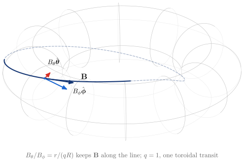
vaft.diagram.field_line_pitch()A field line on a toroidal surface and its field $\mathbf B = B_\phi\hat{\boldsymbol\phi} + B_\theta\hat{\boldsymbol\theta}$.
vaft.diagram.field_line_pitch(q=1.0, *, labels=True)Show source vaft/diagram/_tokamak_geometry.py, lines 569–625
def field_line_pitch(q: float = 1.0, *, labels: bool = True) -> Diagram:
    r"""A field line on a toroidal surface and its field $\mathbf B = B_\phi\hat{\boldsymbol\phi} + B_\theta\hat{\boldsymbol\theta}$.

    The line $\theta = \phi/q$ is followed for one toroidal transit; at one
    point the toroidal and poloidal components are drawn with
    $B_\theta/B_\phi = r/(qR)$, the ratio that keeps $\mathbf B$ tangent to
    the line, so their sum is the line's direction. Small $q$ makes the pitch
    visible; the default is $q = 1$.
    """
    try:
        q = float(q)
    except (TypeError, ValueError):
        raise ValueError(f"q must be a number, not {q!r}") from None
    if not (math.isfinite(q) and 0.5 <= q <= 5.0):
        raise ValueError(f"q must lie in [0.5, 5], not {q!r}")
    labels = _check_labels(labels)
    phi_cut = _camera_cut()
    items: List = _torus_wireframe()
    phi = np.linspace(phi_cut, phi_cut + 2.0 * math.pi, 1201)
    theta = 0.35 + (phi - phi_cut) / q
    line = _torus(_A, theta, phi)
    items += split(_p3(line), _visible(_torus_normal(theta, phi), line), "field line", "field line hidden",
                   "field_line")
    # the point: a visible stretch a little way along the line
    normal = _torus_normal(theta, phi)
    visible = _visible(normal, line)
    view, _, _ = camera()
    facing = np.where(visible, normal @ view, -np.inf)
    facing[:20] = facing[-20:] = -np.inf  # keep the tangent's neighbours on the line
    j = int(np.argmax(facing))  # the most camera-facing visible point
    P, th, ph = line[j], theta[j], phi[j]
    R = _R0 + _A * math.cos(th)
    phi_hat = np.array([-math.sin(ph), math.cos(ph), 0.0])
    theta_hat = np.array([-math.sin(th) * math.cos(ph), -math.sin(th) * math.sin(ph), math.cos(th)])
    B_phi = 1.2
    B_theta = B_phi * _A / (q * R)
    B = B_phi * phi_hat + B_theta * theta_hat
    tangent = (line[j + 1] - line[j - 1]) / np.linalg.norm(line[j + 1] - line[j - 1])
    items += [
        Arrow(tuple(_p3(P)), tuple(_p3(P + B_phi * phi_hat)), "drift ion", role="B_phi"),
        Arrow(tuple(_p3(P)), tuple(_p3(P + B_theta * theta_hat)), "drift", role="B_theta"),
        Arrow(tuple(_p3(P)), tuple(_p3(P + B)), "field vector", role="B"),
        Marker(tuple(_p3(P)), "o", "opoint", role="B"),
    ]
    if labels:
        items += [
            Label(tuple(_p3(P + 1.08 * B_phi * phi_hat)), "$B_\\phi\\hat{\\boldsymbol\\phi}$", "small label",
                  anchor="west", role="B_phi"),
            Label(tuple(_p3(P + 1.3 * B_theta * theta_hat) + np.array([0.0, 0.1])),
                  "$B_\\theta\\hat{\\boldsymbol\\theta}$", "small label", anchor="south", role="B_theta"),
            Label(tuple(_p3(P + 1.05 * B) + np.array([0.1, 0.1])), "$\\mathbf B$", "label", anchor="south west",
                  role="B"),
            _note(f"$B_\\theta/B_\\phi = r/(qR)$ keeps $\\mathbf B$ along the line; $q = {q:g}$, one toroidal transit",
                  float(_p3(np.zeros(3))[0]), _below(items)),
        ]
    model = {"q": q, "field_line": line, "point": P, "B": B, "tangent": tangent, "B_theta_over_B_phi": B_theta / B_phi}
    return Diagram("field_line_pitch", Scene(tuple(items)), model=model)
Formats .svg .tex .pdf the SVG above is committed; build the others locally
import vaft.diagram

d = vaft.diagram.field_line_pitch()
d.tikz  # the TikZ document as text
d.save("field_line_pitch.svg")  # rendered vector image, the canonical artifact; needs latex, dvisvgm
d.save("field_line_pitch.tex")  # the complete TikZ document, the text source
d.save("field_line_pitch.pdf")  # vector PDF; needs pdflatex
Toroidicity and TF ripple, one concept per diagram
Module vaft.diagram._ripple
trapped_and_passing_orbits
1 asset
source
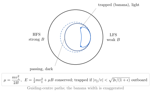
vaft.diagram.trapped_and_passing_orbits()The $1/R$ mirror: passing orbits go round, trapped ones bounce as bananas.
vaft.diagram.trapped_and_passing_orbits(*, labels=True)Show source vaft/diagram/_ripple.py, lines 84–133
def trapped_and_passing_orbits(*, labels: bool = True) -> Diagram:
    r"""The $1/R$ mirror: passing orbits go round, trapped ones bounce as bananas.

    With $\mu = mv_\perp^2/(2B)$ and $E = \tfrac12 mv_\parallel^2 + \mu B$ conserved
    (``parallel_speed_from_mu``) in $B \propto 1/R$ (``vacuum_toroidal_field``),
    a particle launched outboard with small pitch reflects before the inboard
    side; one with large pitch passes. The guiding centre's radial excursion,
    proportional to $v_\parallel$, turns the trapped path into a banana; its
    width is drawn schematically.
    """
    labels = _check_labels(labels)
    epsilon = _R_ORBIT / _R0
    boundary_pitch = math.sqrt(2 * epsilon / (1 + epsilon))  # B_max/B_min = (1 + eps)/(1 - eps)
    orbits = {"trapped": _guiding_centre_orbit(0.5 * boundary_pitch),
              "passing": _guiding_centre_orbit(1.15 * boundary_pitch)}
    theta = np.linspace(0.0, 2.0 * math.pi, 241)
    items: List = [
        Polyline.of(np.stack([_A * np.cos(theta), _A * np.sin(theta)], -1) * _CM, "lcfs", role="boundary", closed=True),
        Polyline.of(np.stack([_R_ORBIT * np.cos(theta), _R_ORBIT * np.sin(theta)], -1) * _CM, "rational",
                    role="flux_surface", closed=True),
    ]
    for name, style in (("passing", "orbit electron"), ("trapped", "orbit ion")):
        o = orbits[name]
        items.append(Polyline.of(np.stack([o["R"] - _R0, o["Z"]], -1) * _CM, style, role=f"orbit_{name}",
                                 closed=not o["trapped"]))
    # the bounce points are the banana's own tips, where v_par = 0
    t = orbits["trapped"]
    for i in (int(np.argmax(t["theta"])), int(np.argmin(t["theta"]))):
        items.append(Marker(((t["R"][i] - _R0) * _CM, t["Z"][i] * _CM), "o", "opoint", role="bounce_point"))
    if labels:
        top = _A * _CM
        items += [
            Label((-top - 0.2, 0.0), "HFS\\\\ strong $B$", "small label,align=center", anchor="east", role="hfs"),
            Label((top + 0.2, 0.0), "LFS\\\\ weak $B$", "small label,align=center", anchor="west", role="lfs"),
            Polyline.of([((t["R"][int(np.argmax(t["theta"]))] - _R0) * _CM, t["Z"][int(np.argmax(t["theta"]))] * _CM),
                         (0.75 * top, 1.05 * top)], "leader line", role="orbit_trapped"),
            Label((0.75 * top + 0.05, 1.05 * top), "trapped (banana), light", "small label", anchor="south west",
                  role="orbit_trapped"),
            Polyline.of([((orbits["passing"]["R"].min() - _R0) * _CM, -0.1),
                         (-0.75 * top, -1.05 * top)], "leader line", role="orbit_passing"),
            Label((-0.75 * top - 0.05, -1.05 * top), "passing, dark", "small label", anchor="north east",
                  role="orbit_passing"),
            Label((0.0, -top - 0.75),
                  "$\\mu = \\dfrac{mv_\\perp^2}{2B}$, $\\ E = \\tfrac12 mv_\\parallel^2 + \\mu B$ conserved; "
                  "trapped if $|v_\\parallel/v| < \\sqrt{2\\epsilon/(1 + \\epsilon)}$ outboard",
                  "formula box", anchor="north", role="equations"),
            _note("Guiding-centre paths; the banana width is exaggerated", 0.0, -top - 1.8),
        ]
    model = {"orbits": orbits, "epsilon": epsilon, "boundary_pitch": boundary_pitch}
    return Diagram("trapped_and_passing_orbits", Scene(tuple(items)), model=model)
Formats .svg .tex .pdf the SVG above is committed; build the others locally
import vaft.diagram

d = vaft.diagram.trapped_and_passing_orbits()
d.tikz  # the TikZ document as text
d.save("trapped_and_passing_orbits.svg")  # rendered vector image, the canonical artifact; needs latex, dvisvgm
d.save("trapped_and_passing_orbits.tex")  # the complete TikZ document, the text source
d.save("trapped_and_passing_orbits.pdf")  # vector PDF; needs pdflatex
Formula functions referenced:
equilibrium.vacuum_toroidal_field, particle.parallel_speed_from_mu
toroidal_field_ripple
1 asset
source
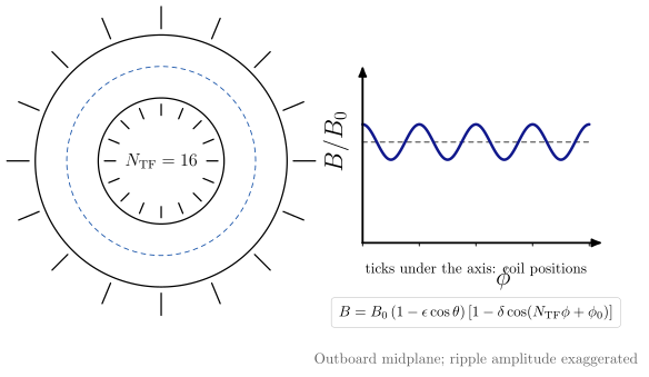
vaft.diagram.toroidal_field_ripple()$N_\mathrm{TF}$ discrete coils corrugate $B(\phi)$ around the smooth $1/R$ field.
vaft.diagram.toroidal_field_ripple(n_tf=16, *, labels=True)Show source vaft/diagram/_ripple.py, lines 141–189
def toroidal_field_ripple(n_tf: int = 16, *, labels: bool = True) -> Diagram:
    r"""$N_\mathrm{TF}$ discrete coils corrugate $B(\phi)$ around the smooth $1/R$ field.

    Left, the torus from above with the coils' legs; right, the outboard
    midplane field of ``toroidal_ripple_field`` over a quarter turn: smooth
    $1 - \epsilon$ and rippled, maximal under each coil and minimal between.
    The ripple amplitude is exaggerated.
    """
    if isinstance(n_tf, bool) or not isinstance(n_tf, (int, np.integer)) or not 4 <= n_tf <= 36:
        raise ValueError(f"n_tf must be an integer from 4 to 36, not {n_tf!r}")
    labels = _check_labels(labels)
    epsilon, delta = 0.3, 0.02
    # top view
    scale = 0.75
    items: List = []
    t = np.linspace(0.0, 2.0 * math.pi, 241)
    for rr, style in ((_R0 - _A, "lcfs"), (_R0 + _A, "lcfs"), (_R0, "rational")):
        items.append(Polyline.of(np.stack([rr * np.cos(t), rr * np.sin(t)], -1) * scale, style, role="plasma",
                                 closed=True))
    coils = 2.0 * math.pi * np.arange(n_tf) / n_tf
    for c in coils:
        for r0, r1 in ((_R0 - _A - 0.55, _R0 - _A - 0.2), (_R0 + _A + 0.2, _R0 + _A + 0.9)):
            items.append(Polyline.of([(r0 * scale * math.cos(c), r0 * scale * math.sin(c)),
                                      (r1 * scale * math.cos(c), r1 * scale * math.sin(c))], "machine", role="coil"))
    # the field along phi on the outboard midplane, a quarter turn
    offset = (_R0 + _A + 1.6) * scale + 0.6
    phi = np.linspace(0.0, 0.5 * math.pi, 801)
    B = toroidal_ripple_field(1.0, epsilon, 0.0, delta, n_tf, phi, phase=math.pi)  # maxima under coils at phi_k
    chart = Chart(x_range=(0.0, 0.5 * math.pi), y_range=(0.62, 0.75))
    chart.curves["rippled"] = np.stack([phi, B], -1)
    chart.curves["smooth"] = np.array([[0.0, 1 - epsilon], [0.5 * math.pi, 1 - epsilon]])
    ticks = tuple(c for c in coils if c <= 0.5 * math.pi + 1e-9)
    scene = render_chart(chart, x_label="$\\phi$", y_label="$B/B_0$",
                         curve_styles={"smooth": "approx", "rippled": "boundary"}, region_text={},
                         x_ticks=ticks, x_tick_text=tuple("" for _ in ticks))
    items += list(scene.transformed(scale=0.6, offset=(offset, -0.3 * CHART_HEIGHT)).items)
    if labels:
        items += [
            Label((0.0, 0.0), f"$N_\\mathrm{{TF}} = {n_tf}$", "label", anchor="center", role="coil"),
            Label((offset + 0.3 * CHART_WIDTH, -0.3 * CHART_HEIGHT - 0.35), "ticks under the axis: coil positions",
                  "small label", anchor="north", role="coil"),
            Label((offset + 0.3 * CHART_WIDTH, -0.3 * CHART_HEIGHT - 1.3),
                  f"$\\displaystyle {formula_equation(toroidal_ripple_field)}$", "formula box", anchor="north",
                  role="equations"),
            _note("Outboard midplane; ripple amplitude exaggerated", offset + 0.3 * CHART_WIDTH,
                  -0.3 * CHART_HEIGHT - 2.5),
        ]
    model = {"n_tf": n_tf, "coils": coils, "phi": phi, "B": B, "epsilon": epsilon, "delta": delta}
    return Diagram("toroidal_field_ripple", Scene(tuple(items)), model=model)
Formats .svg .tex .pdf the SVG above is committed; build the others locally
import vaft.diagram

d = vaft.diagram.toroidal_field_ripple()
d.tikz  # the TikZ document as text
d.save("toroidal_field_ripple.svg")  # rendered vector image, the canonical artifact; needs latex, dvisvgm
d.save("toroidal_field_ripple.tex")  # the complete TikZ document, the text source
d.save("toroidal_field_ripple.pdf")  # vector PDF; needs pdflatex
Formula functions referenced:
ripple.toroidal_ripple_field
ripple_well_formation
1 asset
source
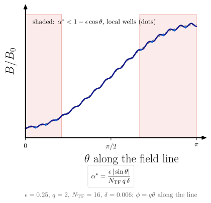
vaft.diagram.ripple_well_formation()Along a field line the ripple makes local wells where $\alpha^* < 1$.
vaft.diagram.ripple_well_formation(*, labels=True)Show source vaft/diagram/_ripple.py, lines 197–252
def ripple_well_formation(*, labels: bool = True) -> Diagram:
    r"""Along a field line the ripple makes local wells where $\alpha^* < 1$.

    $B$ along $\phi = q\theta$ from ``toroidal_ripple_field`` rides on the
    smooth toroidal slope; where ``ripple_well_parameter`` is below 1 --
    near the midplanes, where that slope vanishes -- the corrugation has
    local minima that can trap particles.
    """
    labels = _check_labels(labels)
    eps, q, n, delta = 0.25, 2.0, 16, 0.006
    theta = np.linspace(0.0, math.pi, 4001)
    B = toroidal_ripple_field(1.0, eps, theta, delta, n, q * theta)
    # alpha* is first order; for this multiplicative field wells form where alpha* < 1 - eps cos(theta)
    alpha = ripple_well_parameter(eps, theta, q, delta, n) / (1.0 - eps * np.cos(theta))
    minima = np.flatnonzero((B[1:-1] < B[:-2]) & (B[1:-1] < B[2:])) + 1
    chart = Chart(x_range=(0.0, math.pi), y_range=(0.7, 1.3))
    chart.curves["B"] = np.stack([theta, B], -1)
    chart.curves["smooth"] = np.stack([theta, 1.0 - eps * np.cos(theta)], -1)
    chart.parameters.update({"epsilon": eps, "q": q, "n_tf": n, "delta": delta})
    # the alpha* < 1 bands, shaded under the curve
    inside = alpha < 1.0
    edges = np.flatnonzero(np.diff(inside.astype(int)))
    starts = [0] + list(edges + 1) if inside[0] else list(edges + 1)
    bands = []
    for s0 in starts:
        if not inside[s0]:
            continue
        s1 = s0
        while s1 + 1 < len(inside) and inside[s1 + 1]:
            s1 += 1
        bands.append((float(theta[s0]), float(theta[s1])))
    scene = render_chart(chart, x_label="$\\theta$ along the field line", y_label="$B/B_0$",
                         curve_styles={"smooth": "approx", "B": "boundary"}, region_text={},
                         x_ticks=(0.0, 0.5 * math.pi, math.pi), x_tick_text=("$0$", "$\\pi/2$", "$\\pi$"))
    items: List = []
    for a0, a1 in bands:
        x0, x1 = chart.to_cm(np.array([[a0, 0.7], [a1, 0.7]]))[:, 0]
        items.append(Polyline.of([(x0, 0.0), (x1, 0.0), (x1, CHART_HEIGHT), (x0, CHART_HEIGHT)], "layer",
                                 role="ripple_well_region", closed=True))
    items += list(scene.items)
    for i in minima:
        items.append(Marker(tuple(chart.to_cm(np.array([theta[i], B[i]]))), "o", "opoint", role="ripple_well"))
    if labels:
        items += [
            Label((0.25, CHART_HEIGHT - 0.1), "shaded: $\\alpha^* < 1 - \\epsilon\\cos\\theta$, local wells (dots)",
                  "small label",
                  anchor="north west", role="ripple_well_region"),
            Label((CHART_WIDTH / 2, -1.45), f"$\\displaystyle {formula_equation(ripple_well_parameter)}$",
                  "formula box", anchor="north", role="equations"),
            _note(f"$\\epsilon = {eps:g}$, $q = {q:g}$, $N_\\mathrm{{TF}} = {n}$, $\\delta = {delta:g}$; "
                  "$\\phi = q\\theta$ along the line", CHART_WIDTH / 2, -2.75),
        ]
    model = chart
    chart.parameters["bands"] = bands
    chart.parameters["minima"] = theta[minima]
    return Diagram("ripple_well_formation", Scene(tuple(items)), model=model)
Formats .svg .tex .pdf the SVG above is committed; build the others locally
import vaft.diagram

d = vaft.diagram.ripple_well_formation()
d.tikz  # the TikZ document as text
d.save("ripple_well_formation.svg")  # rendered vector image, the canonical artifact; needs latex, dvisvgm
d.save("ripple_well_formation.tex")  # the complete TikZ document, the text source
d.save("ripple_well_formation.pdf")  # vector PDF; needs pdflatex
Formula functions referenced:
ripple.ripple_well_parameter, ripple.toroidal_ripple_field
stochastic_ripple_orbit
1 asset
source
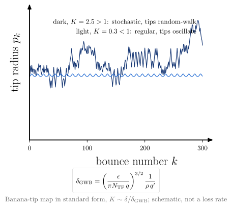
vaft.diagram.stochastic_ripple_orbit()Ripple kicks at successive banana tips decorrelate above the GWB threshold.
vaft.diagram.stochastic_ripple_orbit(*, labels=True)Show source vaft/diagram/_ripple.py, lines 278–314
def stochastic_ripple_orbit(*, labels: bool = True) -> Diagram:
    r"""Ripple kicks at successive banana tips decorrelate above the GWB threshold.

    Each bounce the ripple shifts the banana tip radially by a step $\propto \delta$
    whose sign depends on the tip's ripple phase; the tip's toroidal
    precession then depends on its new radius. Written as a map of the tips it
    is the standard map, $p_{k+1} = p_k + K\sin x_k$, $x_{k+1} = x_k + p_{k+1}$,
    with $K$ playing $\delta/\delta_\mathrm{GWB}$ (``gwb_stochasticity_parameter``;
    the order-one factor is convention). Below $K \approx 1$ the tip oscillates
    about its start; above it random-walks out.
    """
    labels = _check_labels(labels)
    steps = 300
    regular = _tip_map(0.3, steps)
    stochastic = _tip_map(2.5, steps)
    k = np.arange(steps + 1, dtype=float)
    span = float(max(np.abs(regular).max(), np.abs(stochastic).max()))
    chart = Chart(x_range=(0.0, float(steps)), y_range=(-1.1 * span, 1.1 * span))
    chart.curves["regular"] = np.stack([k, regular], -1)
    chart.curves["stochastic"] = np.stack([k, stochastic], -1)
    chart.parameters.update({"K_regular": 0.3, "K_stochastic": 2.5})
    scene = render_chart(chart, x_label="bounce number $k$", y_label="tip radius $p_k$",
                         curve_styles={"stochastic": "orbit electron", "regular": "orbit ion"}, region_text={},
                         x_ticks=(0.0, 100.0, 200.0, 300.0))
    items: List = []
    if labels:
        items += [
            Label((CHART_WIDTH - 0.2, CHART_HEIGHT - 0.1), "dark, $K = 2.5 > 1$: stochastic, tips random-walk",
                  "small label", anchor="north east", role="stochastic"),
            Label((CHART_WIDTH - 0.2, CHART_HEIGHT - 0.6), "light, $K = 0.3 < 1$: regular, tips oscillate",
                  "small label", anchor="north east", role="regular"),
            Label((CHART_WIDTH / 2, -1.45), f"$\\displaystyle {formula_equation(gwb_stochastic_threshold)}$",
                  "formula box", anchor="north", role="equations"),
            _note("Banana-tip map in standard form, $K \\sim \\delta/\\delta_\\mathrm{GWB}$; schematic, not a loss rate",
                  CHART_WIDTH / 2, -2.8),
        ]
    return Diagram("stochastic_ripple_orbit", scene + Scene(tuple(items)), model=chart)
Formats .svg .tex .pdf the SVG above is committed; build the others locally
import vaft.diagram

d = vaft.diagram.stochastic_ripple_orbit()
d.tikz  # the TikZ document as text
d.save("stochastic_ripple_orbit.svg")  # rendered vector image, the canonical artifact; needs latex, dvisvgm
d.save("stochastic_ripple_orbit.tex")  # the complete TikZ document, the text source
d.save("stochastic_ripple_orbit.pdf")  # vector PDF; needs pdflatex
Formula functions referenced:
ripple.gwb_stochastic_threshold
Guiding-centre invariants and toroidal symmetry
Module vaft.diagram._guiding_center
guiding_center_invariants
1 asset
source
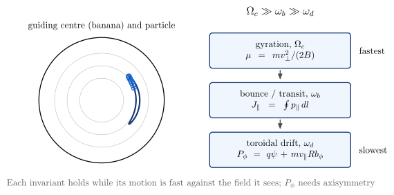
vaft.diagram.guiding_center_invariants()Gyration, bounce and toroidal drift, and the invariant each carries.
vaft.diagram.guiding_center_invariants(*, labels=True)Show source vaft/diagram/_guiding_center.py, lines 162–211
def guiding_center_invariants(*, labels: bool = True) -> Diagram:
    r"""Gyration, bounce and toroidal drift, and the invariant each carries.

    Left, a trapped guiding centre (the banana of ``banana_orbit``) and, along
    part of it, the particle gyrating about it -- Larmor radius exaggerated.
    Right, the three motions from fastest to slowest with their invariants:
    $\mu = mv_\perp^2/(2B)$ for gyration, $J_\parallel = \oint p_\parallel\,dl$
    for the bounce, $P_\phi$ for the toroidal drift. Each is conserved only
    while its motion is fast against changes of the field it sees
    ($\Omega_c \gg \omega_b \gg \omega_d$); $P_\phi$ needs axisymmetry.
    """
    labels = _check_labels(labels)
    orbit = banana_orbit()
    items: List = []
    _surfaces(items)
    gc = _xy(orbit["R"], orbit["Z"])
    items.append(Polyline.of(gc, "field line", role="guiding_center", closed=True))
    # the particle about part of the upper leg: guiding centre plus a gyration, schematic radius
    k = np.arange(len(gc) // 16, len(gc) // 4)
    phase = np.linspace(0.0, 9.0 * 2.0 * math.pi, len(k))
    rho = 0.1
    particle = gc[k] + rho * np.stack([np.cos(phase), np.sin(phase)], -1)
    items.append(Polyline.of(particle, "orbit ion", role="particle_orbit"))
    x0 = 1.6 * _A * _CM
    rows = [
        ("gyro", "mu", "gyration, $\\Omega_c$\\\\ $\\mu = mv_\\perp^2/(2B)$"),
        ("bounce", "j_parallel", "bounce / transit, $\\omega_b$\\\\ $J_\\parallel = \\oint p_\\parallel\\,dl$"),
        ("drift", "p_phi", "toroidal drift, $\\omega_d$\\\\ $P_\\phi = q\\psi + mv_\\parallel Rb_\\phi$"),
    ]
    boxes = []
    for i, (motion, invariant, text) in enumerate(rows):
        b = box(x0 + 3.0, 1.9 - 1.9 * i, 5.4, 1.35, text, role=f"invariant:{invariant}", latex=True)
        boxes.append(b)
        items += list(b.items)
        items.append(Label((x0 + 5.9, 1.9 - 1.9 * i), {"gyro": "fastest", "bounce": "", "drift": "slowest"}[motion]
                           if labels else "", "small label", anchor="west", role=f"motion:{motion}"))
    items += [connector(boxes[0], boxes[1], role="ordering"), connector(boxes[1], boxes[2], role="ordering")]
    if labels:
        top = _A * _CM
        items += [
            Label((0.0, top + 0.15), "guiding centre (banana) and particle", "small label", anchor="south",
                  role="guiding_center"),
            Label((x0 + 3.0, 3.1), "$\\Omega_c \\gg \\omega_b \\gg \\omega_d$", "label", anchor="south",
                  role="ordering"),
            Label((0.5 * (x0 + 3.0), -top - 0.5),
                  "Each invariant holds while its motion is fast against the field it sees; $P_\\phi$ needs axisymmetry",
                  "note", anchor="north", role="note"),
        ]
    model = {"orbit": orbit, "rho": rho, "invariants": ("mu", "j_parallel", "p_phi")}
    return Diagram("guiding_center_invariants", Scene(tuple(items)), model=model)
Formats .svg .tex .pdf the SVG above is committed; build the others locally
import vaft.diagram

d = vaft.diagram.guiding_center_invariants()
d.tikz  # the TikZ document as text
d.save("guiding_center_invariants.svg")  # rendered vector image, the canonical artifact; needs latex, dvisvgm
d.save("guiding_center_invariants.tex")  # the complete TikZ document, the text source
d.save("guiding_center_invariants.pdf")  # vector PDF; needs pdflatex
Formula functions referenced:
equilibrium.vacuum_toroidal_field, particle.guiding_center_toroidal_momentum, particle.parallel_speed_from_mu
canonical_toroidal_momentum
1 asset
source
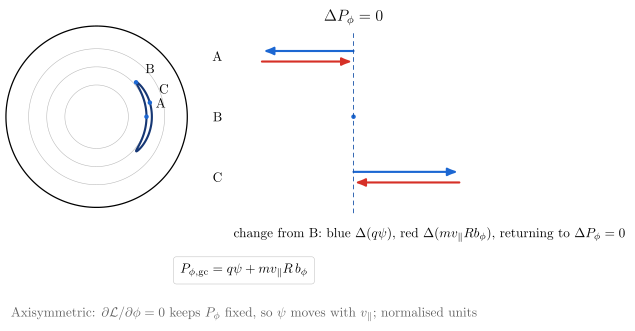
vaft.diagram.canonical_toroidal_momentum()$P_\phi = q\psi + mv_\parallel Rb_\phi$ along one banana: the parts trade, the sum stays.
vaft.diagram.canonical_toroidal_momentum(phase=0.45, *, labels=True)Show source vaft/diagram/_guiding_center.py, lines 219–285
def canonical_toroidal_momentum(phase: float = 0.45, *, labels: bool = True) -> Diagram:
    r"""$P_\phi = q\psi + mv_\parallel Rb_\phi$ along one banana: the parts trade, the sum stays.

    Three points of the orbit of ``banana_orbit`` -- the outboard start, the
    upper bounce tip and the point a fraction ``phase`` of the way round --
    with bars of their flux part $q\psi$ and mechanical part $mv_\parallel Rb_\phi$
    from ``guiding_center_toroidal_momentum``. Where $v_\parallel$ falls the flux
    part rises: the guiding centre crosses surfaces, which is the orbit width.
    ``phase`` is the state coordinate a later animation would step.
    """
    try:
        phase = float(phase)
    except (TypeError, ValueError):
        raise ValueError(f"phase must be a number in [0, 1), not {phase!r}") from None
    if not 0.0 <= phase < 1.0:
        raise ValueError(f"phase must lie in [0, 1), not {phase!r}")
    labels = _check_labels(labels)
    orbit = banana_orbit()
    n = len(orbit["theta"])
    tip = int(np.argmax(orbit["theta"]))  # the upper bounce tip, v_par = 0 there
    picks = {"A": 0, "B": tip, "C": int(round(phase * (n - 1)))}
    items: List = []
    _surfaces(items)
    items.append(Polyline.of(_xy(orbit["R"], orbit["Z"]), "field line", role="guiding_center", closed=True))
    parts = {}
    for name, i in picks.items():
        flux = float(orbit["psi"][i])
        mech = float(orbit["v_par"][i] * orbit["R"][i])
        total = guiding_center_toroidal_momentum(1.0, 1.0, orbit["v_par"][i], orbit["R"][i], 1.0, orbit["psi"][i])
        parts[name] = {"flux": flux, "mechanical": mech, "P_phi": total}
        at = tuple(_xy(orbit["R"][i], orbit["Z"][i]))
        items.append(Marker(at, "o", "opoint", role=f"point:{name}"))
        if labels:
            items.append(Label((at[0] + 0.12, at[1] + 0.12), name, "small label", anchor="south west",
                               role=f"point:{name}"))
    # the bars: each point's change of the two parts from the bounce tip B, where v_par = 0.
    # They are equal and opposite -- the sum, P_phi, does not move.
    x0 = 1.5 * _A * _CM + 3.2
    ref = parts["B"]
    changes = {k: (v["flux"] - ref["flux"], v["mechanical"] - ref["mechanical"]) for k, v in parts.items()}
    scale = 2.8 / max(max(abs(a), abs(b)) for a, b in changes.values())
    for j, (name, (d_flux, d_mech)) in enumerate(changes.items()):
        y = 1.6 - 1.6 * j
        if abs(d_flux) * scale > 0.05:  # at B both changes are zero: nothing to draw
            items += [
                Arrow((x0, y + 0.14), (x0 + d_flux * scale, y + 0.14), "drift ion", role=f"bar:flux:{name}"),
                Arrow((x0 + d_flux * scale, y - 0.14), (x0 + (d_flux + d_mech) * scale, y - 0.14), "drift",
                      role=f"bar:mechanical:{name}"),
            ]
        else:
            items.append(Marker((x0, y), "o", "opoint", role=f"bar:flux:{name}"))
        if labels:
            items.append(Label((x0 - 3.35, y), name, "small label", anchor="east", role=f"bar:{name}"))
    items.append(Polyline.of([(x0, 2.2), (x0, -2.2 - 0.4)], "rational", role="p_phi_level"))
    if labels:
        top = _A * _CM
        items += [
            Label((x0, 2.3), "$\\Delta P_\\phi = 0$", "label", anchor="south", role="p_phi_level"),
            Label((x0 - 3.3, -2.8), "change from B: blue $\\Delta(q\\psi)$, red $\\Delta(mv_\\parallel Rb_\\phi)$, returning to $\\Delta P_\\phi = 0$",
                  "small label", anchor="north west", role="bar:key"),
            Label((0.5 * (x0 + 1.0), -top - 1.3), f"$\\displaystyle {formula_equation(guiding_center_toroidal_momentum)}$",
                  "formula box", anchor="north", role="equations"),
            _note_label("Axisymmetric: $\\partial\\mathcal{L}/\\partial\\phi = 0$ keeps $P_\\phi$ fixed, so $\\psi$ moves "
                        "with $v_\\parallel$; normalised units", 0.5 * (x0 + 1.0), -top - 2.5),
        ]
    model = {"orbit": orbit, "points": picks, "parts": parts, "changes": changes, "phase": phase}
    return Diagram("canonical_toroidal_momentum", Scene(tuple(items)), model=model)
Formats .svg .tex .pdf the SVG above is committed; build the others locally
import vaft.diagram

d = vaft.diagram.canonical_toroidal_momentum()
d.tikz  # the TikZ document as text
d.save("canonical_toroidal_momentum.svg")  # rendered vector image, the canonical artifact; needs latex, dvisvgm
d.save("canonical_toroidal_momentum.tex")  # the complete TikZ document, the text source
d.save("canonical_toroidal_momentum.pdf")  # vector PDF; needs pdflatex
Formula functions referenced:
equilibrium.vacuum_toroidal_field, particle.guiding_center_toroidal_momentum, particle.parallel_speed_from_mu
toroidal_symmetry_breaking
1 asset
source
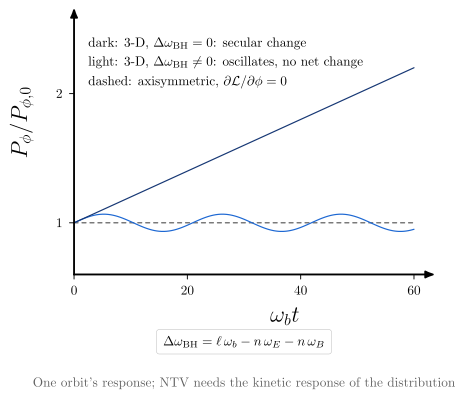
vaft.diagram.toroidal_symmetry_breaking()Axisymmetry keeps $P_\phi$; a 3-D field changes it, secularly only at resonance.
vaft.diagram.toroidal_symmetry_breaking(*, labels=True)Show source vaft/diagram/_guiding_center.py, lines 297–336
def toroidal_symmetry_breaking(*, labels: bool = True) -> Diagram:
    r"""Axisymmetry keeps $P_\phi$; a 3-D field changes it, secularly only at resonance.

    With a toroidal-$n$ perturbation, $dP_\phi/dt \propto \cos(\Delta\omega_\mathrm{BH}t)$
    along the orbit, $\Delta\omega_\mathrm{BH}$ from ``bounce_harmonic_detuning``:
    away from resonance $P_\phi$ oscillates with no net change, at
    $\Delta\omega_\mathrm{BH} = 0$ it drifts linearly. The drift of one orbit
    is not NTV; torque and transport need the kinetic response of the whole
    distribution (#1111).
    """
    labels = _check_labels(labels)
    t = np.linspace(0.0, 60.0, 1201)
    kick = 0.02
    detuned = bounce_harmonic_detuning(1.0, 0.25, 0.1, l=1, n=2)  # 1 - 0.7 = 0.3: three periods shown
    resonant = bounce_harmonic_detuning(1.0, 0.375, 0.125, l=1, n=2)  # exactly 0
    curves = {"axisymmetric": np.ones_like(t),
              "non_resonant": 1.0 + kick * np.sin(detuned * t) / detuned,
              "resonant": 1.0 + kick * t}
    chart = Chart(x_range=(0.0, 60.0), y_range=(0.6, 2.5))
    for name, c in curves.items():
        chart.curves[name] = np.stack([t, c], -1)
    chart.parameters.update({"detuning_non_resonant": detuned, "detuning_resonant": resonant, "kick": kick})
    scene = render_chart(chart, x_label="$\\omega_b t$", y_label="$P_\\phi/P_{\\phi,0}$",
                         curve_styles={"axisymmetric": "approx", "non_resonant": "orbit ion", "resonant": "orbit electron"},
                         region_text={}, x_ticks=(0.0, 20.0, 40.0, 60.0), y_ticks=(1.0, 2.0))
    items: List = []
    if labels:
        items += [
            Label((0.25, CHART_HEIGHT - 0.1), "dark: 3-D, $\\Delta\\omega_\\mathrm{BH} = 0$: secular change",
                  "small label", anchor="north west", role="resonant"),
            Label((0.25, CHART_HEIGHT - 0.6), "light: 3-D, $\\Delta\\omega_\\mathrm{BH} \\ne 0$: oscillates, no net change",
                  "small label", anchor="north west", role="non_resonant"),
            Label((0.25, CHART_HEIGHT - 1.1), "dashed: axisymmetric, $\\partial\\mathcal{L}/\\partial\\phi = 0$",
                  "small label", anchor="north west", role="axisymmetric"),
            Label((CHART_WIDTH / 2, -1.45), f"$\\displaystyle {formula_equation(bounce_harmonic_detuning)}$",
                  "formula box", anchor="north", role="equations"),
            _note_label("One orbit's response; NTV needs the kinetic response of the distribution", CHART_WIDTH / 2,
                        -2.6),
        ]
    return Diagram("toroidal_symmetry_breaking", scene + Scene(tuple(items)), model=chart)
Formats .svg .tex .pdf the SVG above is committed; build the others locally
import vaft.diagram

d = vaft.diagram.toroidal_symmetry_breaking()
d.tikz  # the TikZ document as text
d.save("toroidal_symmetry_breaking.svg")  # rendered vector image, the canonical artifact; needs latex, dvisvgm
d.save("toroidal_symmetry_breaking.tex")  # the complete TikZ document, the text source
d.save("toroidal_symmetry_breaking.pdf")  # vector PDF; needs pdflatex
Formula functions referenced:
particle.bounce_harmonic_detuning
Straight-field-line coordinates: one equilibrium, many angles
Module vaft.diagram._sfl_coordinates
sfl_coordinate_grids
1 asset
source
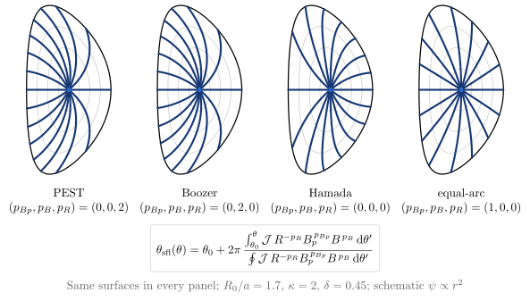
vaft.diagram.sfl_coordinate_grids()PEST, Boozer, Hamada and equal-arc on the same equilibrium: only the angle changes.
vaft.diagram.sfl_coordinate_grids(*, labels=True)Show source vaft/diagram/_sfl_coordinates.py, lines 111–149
def sfl_coordinate_grids(*, labels: bool = True) -> Diagram:
    r"""PEST, Boozer, Hamada and equal-arc on the same equilibrium: only the angle changes.

    Each panel draws the same nested surfaces ($R_0/a = 1.7$, $\kappa = 2$,
    $\delta = 0.45$) and sixteen lines of constant poloidal angle in one
    member of the generalised straight-field-line family
    (``generalized_straight_field_line_angle``). Field lines are straight in
    every one of them; what differs is how the angle is distributed.
    """
    labels = _check_labels(labels)
    radii = (0.25, 0.5, 0.75, 1.0)
    gap = 3.1 * _A * _CM
    items: List = []
    for i, name in enumerate(COORDINATES):
        x0 = i * gap
        theta = np.linspace(0.0, 2.0 * math.pi, 241)
        for r in radii:
            R, Z = _section(r, theta)
            items.append(Polyline.of(_xy(np.stack([R, Z], -1), x0), "lcfs" if r == 1.0 else "surface",
                                     role=f"surface:{name}", closed=True))
        for line in _angle_lines(name):
            items.append(Polyline.of(_xy(line, x0), "field line", role=f"grid:{name}"))
        items.append(Marker((x0, 0.0), "o", "opoint", role=f"surface:{name}"))
        if labels:
            p = COORDINATES[name]
            items.append(Label((x0, -_KAPPA * _A * _CM - 0.3),
                               f"{name}\\\\ $(p_{{Bp}}, p_B, p_R) = ({p[0]:g}, {p[1]:g}, {p[2]:g})$",
                               "small label,align=center", anchor="north", role=f"title:{name}"))
    if labels:
        items += [
            Label((1.5 * gap, -_KAPPA * _A * _CM - 1.5),
                  f"$\\displaystyle {formula_equation(generalized_straight_field_line_angle)}$", "formula box",
                  anchor="north", role="equations"),
            Label((1.5 * gap, -_KAPPA * _A * _CM - 3.0),
                  "Same surfaces in every panel; $R_0/a = 1.7$, $\\kappa = 2$, $\\delta = 0.45$; schematic $\\psi \\propto r^2$",
                  "note", anchor="north", role="note"),
        ]
    model = {"coordinates": dict(COORDINATES), "radii": radii}
    return Diagram("sfl_coordinate_grids", Scene(tuple(items)), model=model)
Formats .svg .tex .pdf the SVG above is committed; build the others locally
import vaft.diagram

d = vaft.diagram.sfl_coordinate_grids()
d.tikz  # the TikZ document as text
d.save("sfl_coordinate_grids.svg")  # rendered vector image, the canonical artifact; needs latex, dvisvgm
d.save("sfl_coordinate_grids.tex")  # the complete TikZ document, the text source
d.save("sfl_coordinate_grids.pdf")  # vector PDF; needs pdflatex
Formula functions referenced:
equilibrium.generalized_straight_field_line_angle, equilibrium.miller_surface, equilibrium.vacuum_toroidal_field
sfl_coordinate_taxonomy
1 asset
source
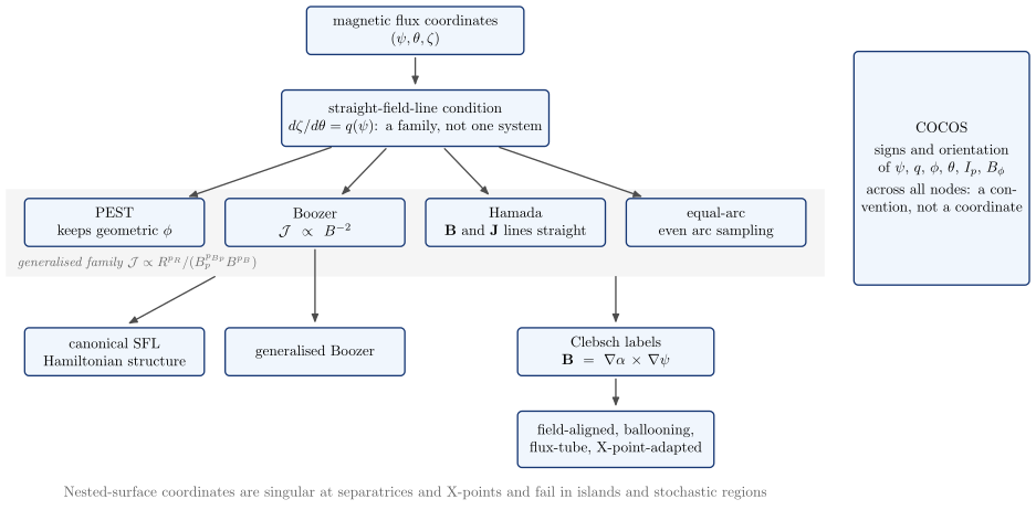
vaft.diagram.sfl_coordinate_taxonomy()Flux coordinates, the straight-field-line condition, and what each named choice fixes.
vaft.diagram.sfl_coordinate_taxonomy(*, labels=True)Show source vaft/diagram/_sfl_coordinates.py, lines 157–216
def sfl_coordinate_taxonomy(*, labels: bool = True) -> Diagram:
    r"""Flux coordinates, the straight-field-line condition, and what each named choice fixes.

    The straight-field-line condition $d\zeta/d\theta = q(\psi)$ leaves a
    freedom that PEST, Boozer, Hamada and equal-arc fix in different ways
    (the generalised family); canonical and generalised-Boozer coordinates
    branch further. Clebsch field-line labels and the field-aligned, ballooning
    and flux-tube coordinates are derived from them. COCOS is a separate
    layer -- orientation and sign conventions -- across all of it, not a
    coordinate choice. Nested-surface coordinates fail at separatrices,
    islands and stochastic regions.
    """
    labels = _check_labels(labels)
    W, H = 4.3, 1.15
    items: List = []
    nodes = {
        "flux": box(0.0, 0.0, 5.2, H, "magnetic flux coordinates\\\\ $(\\psi, \\theta, \\zeta)$", role="node:flux",
                    latex=True),
        "sfl": box(0.0, -2.1, 6.4, 1.35, "straight-field-line condition\\\\ $d\\zeta/d\\theta = q(\\psi)$: a family, "
                   "not one system", role="node:sfl", latex=True),
        "pest": box(-7.2, -4.6, W, H, "PEST\\\\ keeps geometric $\\phi$", role="node:pest", latex=True),
        "boozer": box(-2.4, -4.6, W, H, "Boozer\\\\ $\\mathcal{J} \\propto B^{-2}$", role="node:boozer", latex=True),
        "hamada": box(2.4, -4.6, W, H, "Hamada\\\\ $\\mathbf{B}$ and $\\mathbf{J}$ lines straight",
                      role="node:hamada", latex=True),
        "equal_arc": box(7.2, -4.6, W, H, "equal-arc\\\\ even arc sampling", role="node:equal_arc",
                         latex=True),
        "gen_boozer": box(-2.4, -7.7, W, H, "generalised Boozer", role="node:generalized_boozer"),
        "canonical": box(-7.2, -7.7, W, H, "canonical SFL\\\\ Hamiltonian structure", role="node:canonical",
                         latex=True),
        "clebsch": box(4.8, -7.7, W + 0.4, H, "Clebsch labels\\\\ $\\mathbf{B} = \\nabla\\alpha\\times\\nabla\\psi$",
                       role="node:clebsch", latex=True),
        "aligned": box(4.8, -9.8, W + 0.4, 1.35, "field-aligned, ballooning,\\\\ flux-tube, X-point-adapted",
                       role="node:derived", latex=True),
    }
    items += band(-9.8, 9.8, -5.9, -3.8, role="family")
    items.append(Label((-9.65, -5.85), "generalised family $\\mathcal{J} \\propto R^{p_R}/(B_p^{p_{Bp}}B^{p_B})$",
                       "concept band label", anchor="south west", role="family"))
    for b in nodes.values():
        items += list(b.items)
    for a, b in (("flux", "sfl"), ("sfl", "pest"), ("sfl", "boozer"), ("sfl", "hamada"), ("sfl", "equal_arc"),
                 ("boozer", "gen_boozer"), ("clebsch", "aligned")):
        items.append(connector(nodes[a], nodes[b], role=f"edge:{a}->{b}"))
    # canonical SFL and Clebsch labels come from the family as a whole, not from one member:
    # their arrows leave the band between the member boxes
    for name, gap_x in (("canonical", -4.8), ("clebsch", 4.8)):
        n = nodes[name]
        items.append(Arrow((gap_x, -5.9), (n.x + (0.3 if n.x < gap_x else -0.3 if n.x > gap_x else 0.0),
                                           n.y + 0.5 * n.height + 0.08), "connector", role=f"edge:family->{name}"))
    # COCOS: a convention layer across the whole tree, drawn beside it
    cocos = box(12.6, -3.3, 4.2, 5.6, "COCOS\\\\[3pt] signs and orientation of $\\psi$, $q$, $\\phi$, $\\theta$, "
                "$I_p$, $B_\\phi$\\\\[3pt] across all nodes: a convention, not a coordinate", role="node:cocos",
                latex=True)
    items += list(cocos.items)
    if labels:
        items += [
            Label((0.0, -10.8), "Nested-surface coordinates are singular at separatrices and X-points and fail in islands "
                  "and stochastic regions", "note", anchor="north", role="note"),
        ]
    model = {"nodes": tuple(nodes), "family": tuple(COORDINATES)}
    return Diagram("sfl_coordinate_taxonomy", Scene(tuple(items)), model=model)
Formats .svg .tex .pdf the SVG above is committed; build the others locally
import vaft.diagram

d = vaft.diagram.sfl_coordinate_taxonomy()
d.tikz  # the TikZ document as text
d.save("sfl_coordinate_taxonomy.svg")  # rendered vector image, the canonical artifact; needs latex, dvisvgm
d.save("sfl_coordinate_taxonomy.tex")  # the complete TikZ document, the text source
d.save("sfl_coordinate_taxonomy.pdf")  # vector PDF; needs pdflatex
sfl_fourier_convergence
2 assets
source
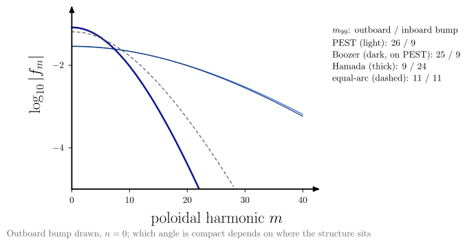
vaft.diagram.sfl_fourier_convergence()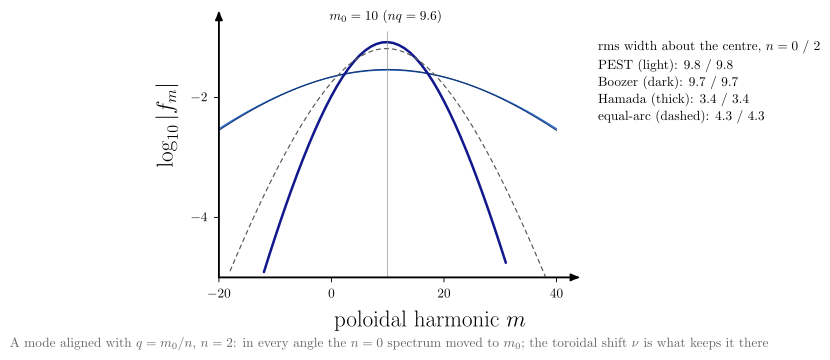
vaft.diagram.sfl_fourier_convergence(n=2)The same physical perturbation has a different poloidal spectrum in each straight-field-line angle.
vaft.diagram.sfl_fourier_convergence(*, n=0, labels=True)Show source vaft/diagram/_sfl_coordinates.py, lines 301–346
def sfl_fourier_convergence(*, n: int = 0, labels: bool = True) -> Diagram:
    r"""The same physical perturbation has a different poloidal spectrum in each straight-field-line angle.

    One outboard-localised perturbation on the $r = 0.8$ surface of the
    grids' equilibrium, expanded in $e^{im\theta}$ for PEST, Boozer, Hamada
    and equal-arc; the legend gives the number of harmonics that carry 99 %
    of its power in each. Where an angle stretches the region the
    perturbation lives in, its spectrum narrows; where it compresses it, the
    spectrum broadens -- the same structure, a different numerical cost.
    With a toroidal mode number ``n`` $\ne 0$ the members other than PEST
    also carry the toroidal shift $\nu$ (``sfl_toroidal_angle_shift``), whose
    $e^{in\nu}$ couples harmonics: their spectra broaden with $n$ while PEST's
    does not.
    """
    labels = _check_labels(labels)
    if isinstance(n, bool) or not isinstance(n, (int, np.integer)) or not 0 <= n <= 8:
        raise ValueError(f"n must be an integer from 0 to 8, not {n!r}")
    if n:
        return _fourier_convergence_shifted(int(n), labels)
    spectra = perturbation_spectra()
    inboard = perturbation_spectra(math.pi)
    m = np.arange(_M_MAX + 1, dtype=float)
    top = max(float(v["amplitude"].max()) for v in spectra.values())
    styles = {"PEST": "orbit ion", "Boozer": "orbit electron", "Hamada": "boundary", "equal-arc": "approx"}
    keys = {"PEST": "light", "Boozer": "dark, on PEST", "Hamada": "thick", "equal-arc": "dashed"}
    # log scale on y, drawn as log10
    chart = Chart(x_range=(0.0, float(_M_MAX) + 0.5), y_range=(-5.0, math.log10(1.5 * top)))
    for name, v in spectra.items():
        chart.curves[name] = np.stack([m, np.log10(np.maximum(v["amplitude"], 1e-6))], -1)
    chart.parameters.update({name: v["m99"] for name, v in spectra.items()})
    chart.parameters["inboard"] = {name: v["m99"] for name, v in inboard.items()}
    scene = render_chart(chart, x_label="poloidal harmonic $m$", y_label="$\\log_{10}|f_m|$",
                         curve_styles=styles, region_text={}, x_ticks=(0.0, 10.0, 20.0, 30.0, 40.0),
                         y_ticks=(-4.0, -2.0))
    items: List = []
    if labels:
        # beside the chart: the steep spectra cross every corner of it
        items.append(Label((CHART_WIDTH + 0.9, CHART_HEIGHT - 0.1), "$m_{99}$: outboard / inboard bump", "small label",
                           anchor="north west", role="legend"))
        for i, (name, v) in enumerate(spectra.items()):
            items.append(Label((CHART_WIDTH + 0.9, CHART_HEIGHT - 0.6 - 0.45 * i),
                               f"{name} ({keys[name]}): {v['m99']} / {inboard[name]['m99']}", "small label",
                               anchor="north west", role=f"legend:{name}"))
        items.append(Label((CHART_WIDTH / 2, -1.45), "Outboard bump drawn, $n = 0$; which angle is compact depends "
                           "on where the structure sits", "note", anchor="north", role="note"))
    return Diagram("sfl_fourier_convergence", scene + Scene(tuple(items)), model=chart)
Formats .svg .tex .pdf the SVG above is committed; build the others locally
import vaft.diagram

d = vaft.diagram.sfl_fourier_convergence()
d.tikz  # the TikZ document as text
d.save("sfl_fourier_convergence.svg")  # rendered vector image, the canonical artifact; needs latex, dvisvgm
d.save("sfl_fourier_convergence.tex")  # the complete TikZ document, the text source
d.save("sfl_fourier_convergence.pdf")  # vector PDF; needs pdflatex
Formula functions referenced:
equilibrium.generalized_straight_field_line_angle, equilibrium.miller_surface, equilibrium.sfl_toroidal_angle_shift, equilibrium.vacuum_toroidal_field
field_line_action_angle
1 asset
source
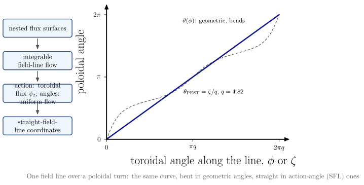
vaft.diagram.field_line_action_angle()Straight-field-line coordinates are the action-angle variables of the field-line flow.
vaft.diagram.field_line_action_angle(*, labels=True)Show source vaft/diagram/_sfl_coordinates.py, lines 391–437
def field_line_action_angle(*, labels: bool = True) -> Diagram:
    r"""Straight-field-line coordinates are the action-angle variables of the field-line flow.

    Left, the chain: nested flux surfaces make the field-line flow
    integrable; its action is the flux $\psi$ and its angles make the flow
    uniform, $\theta = \theta_0 + \iota(\psi)\zeta$ -- the straight-field-line
    coordinates. Right, one field line on the $r = 0.8$ surface of the
    grids' equilibrium, over one poloidal turn: against the geometric angles
    $(\phi, \vartheta)$ it bends, against $(\zeta, \theta_\mathrm{PEST})$ it is the
    straight line of slope $\iota = 1/q$, with $q$ the surface's own.
    """
    labels = _check_labels(labels)
    s = _surface(_R_SPECTRUM)
    q = s["q"]
    theta_p = s["angles"]["PEST"]
    # along the field line d phi = q d theta_PEST, starting at the outboard midplane
    phi = q * theta_p
    R, Z = s["R"], s["Z"]
    polar = np.unwrap(np.arctan2(Z, R - _R0))
    chain = [("surfaces", "nested flux surfaces"), ("integrable", "integrable field-line flow"),
             ("action_angle", "action: toroidal flux $\\psi_t$; angles: uniform flow"), ("sfl", "straight-field-line coordinates")]
    items: List = []
    boxes = {}
    for k, (role, text) in enumerate(chain):
        boxes[role] = box(0.0, 5.6 - 1.7 * k, 3.6, 0.95, text if labels else "", role=role, latex=True)
        items += boxes[role].items
    for a, b in zip(chain, chain[1:]):
        items.append(connector(boxes[a[0]], boxes[b[0]], role=f"{a[0]}->{b[0]}"))
    chart = Chart(x_range=(0.0, 2.0 * math.pi * q), y_range=(0.0, 2.0 * math.pi))
    chart.curves["geometric"] = np.stack([phi, polar - polar[0]], -1)
    chart.curves["straight"] = np.stack([phi, theta_p], -1)
    chart.labels.update({"geometric": (0.62 * 2 * math.pi * q, 0.95 * 2 * math.pi),
                         "straight": (0.62 * 2 * math.pi * q, 0.38 * 2 * math.pi)})
    chart.parameters.update({"q": q, "iota": 1.0 / q, "r": _R_SPECTRUM})
    ticks = [0.0, math.pi, 2.0 * math.pi]
    scene = render_chart(
        chart, x_label="toroidal angle along the line, $\\phi$ or $\\zeta$", y_label="poloidal angle",
        curve_styles={"geometric": "approx", "straight": "boundary"},
        region_text={"geometric": "\\small $\\vartheta(\\phi)$: geometric, bends",
                     "straight": f"\\small $\\theta_\\mathrm{{PEST}} = \\zeta/q$, $q = {q:.2f}$"} if labels else {},
        x_ticks=[0.0, math.pi * q, 2.0 * math.pi * q], x_tick_text=["$0$", "$\\pi q$", "$2\\pi q$"],
        y_ticks=ticks, y_tick_text=["$0$", "$\\pi$", "$2\\pi$"],
        note=("One field line over a poloidal turn: the same curve, bent in geometric angles, straight in "
              "action-angle (SFL) ones" if labels else ""),
    )
    items += list(scene.transformed(offset=(3.6, -0.2)).items)
    return Diagram("field_line_action_angle", Scene(tuple(items)), model=chart)
Formats .svg .tex .pdf the SVG above is committed; build the others locally
import vaft.diagram

d = vaft.diagram.field_line_action_angle()
d.tikz  # the TikZ document as text
d.save("field_line_action_angle.svg")  # rendered vector image, the canonical artifact; needs latex, dvisvgm
d.save("field_line_action_angle.tex")  # the complete TikZ document, the text source
d.save("field_line_action_angle.pdf")  # vector PDF; needs pdflatex
Formula functions referenced:
equilibrium.generalized_straight_field_line_angle, equilibrium.miller_surface, equilibrium.vacuum_toroidal_field
sfl_coordinate_validity
1 asset
source
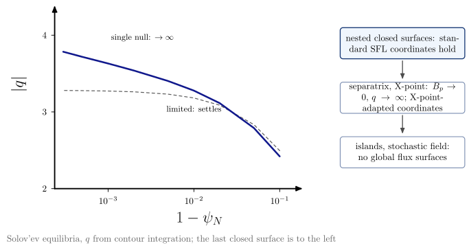
vaft.diagram.sfl_coordinate_validity()Where nested-surface straight-field-line coordinates hold, and where they fail.
vaft.diagram.sfl_coordinate_validity(*, labels=True)Show source vaft/diagram/_sfl_coordinates.py, lines 461–503
def sfl_coordinate_validity(*, labels: bool = True) -> Diagram:
    r"""Where nested-surface straight-field-line coordinates hold, and where they fail.

    Left, computed: $|q|$ toward the last closed surface of a limited and of
    a single-null Solov'ev equilibrium (``calculate_q_profile_from_psi``).
    Limited, $q$ settles; diverted, $B_p \to 0$ at the X-point and $q$ grows
    as $\ln(1 - \psi_N)$ without bound -- the angle $\theta^*$, whose rate is
    $\propto 1/q$ along the line, degenerates there. Right, the three cases:
    nested closed surfaces (valid), a separatrix or X-point (singular, special
    treatment), islands or stochastic fields (no global flux surfaces; see
    ``magnetic_island`` and ``stochastic_layer``).
    """
    labels = _check_labels(labels)
    prof = separatrix_q_profiles()
    x = np.log10(prof["distance"])
    chart = Chart(x_range=(float(x.min()) - 0.1, float(x.max()) + 0.1), y_range=(2.0, 4.2))
    chart.curves["limited"] = np.stack([x, prof["limited"]], -1)
    chart.curves["single_null"] = np.stack([x, prof["single_null"]], -1)
    chart.labels.update({"limited": (-2.0, float(prof["limited"][-4]) - 0.22),
                         "single_null": (-2.6, float(prof["single_null"][-2]) + 0.25)})
    chart.parameters.update({"q_limited_edge": float(prof["limited"][-1]),
                             "q_single_null_edge": float(prof["single_null"][-1])})
    scene = render_chart(
        chart, x_label="$1 - \\psi_N$", y_label="$|q|$",
        curve_styles={"limited": "approx", "single_null": "boundary"},
        region_text={"limited": "\\small limited: settles", "single_null": "\\small single null: $\\to\\infty$"}
        if labels else {},
        x_ticks=[-3.0, -2.0, -1.0], x_tick_text=["$10^{-3}$", "$10^{-2}$", "$10^{-1}$"],
        y_ticks=[2.0, 3.0, 4.0],
        note="Solov'ev equilibria, $q$ from contour integration; the last closed surface is to the left" if labels else "",
    )
    items: List = list(scene.items)
    cases = [("valid", "nested closed surfaces: standard SFL coordinates hold"),
             ("singular", "separatrix, X-point: $B_p \\to 0$, $q \\to \\infty$; X-point-adapted coordinates"),
             ("fails", "islands, stochastic field: no global flux surfaces")]
    boxes = {}
    for k, (role, text) in enumerate(cases):
        boxes[role] = box(CHART_WIDTH + 4.4, CHART_HEIGHT - 0.9 - 2.1 * k, 4.8, 1.2, text if labels else "",
                          style="concept box" if role == "valid" else "concept leaf", role=role, latex=True)
        items += boxes[role].items
    for a, b in (("valid", "singular"), ("singular", "fails")):
        items.append(connector(boxes[a], boxes[b], role=f"{a}->{b}"))
    return Diagram("sfl_coordinate_validity", Scene(tuple(items)), model=chart)
Formats .svg .tex .pdf the SVG above is committed; build the others locally
import vaft.diagram

d = vaft.diagram.sfl_coordinate_validity()
d.tikz  # the TikZ document as text
d.save("sfl_coordinate_validity.svg")  # rendered vector image, the canonical artifact; needs latex, dvisvgm
d.save("sfl_coordinate_validity.tex")  # the complete TikZ document, the text source
d.save("sfl_coordinate_validity.pdf")  # vector PDF; needs pdflatex
coordinates_vs_cocos
1 asset
source
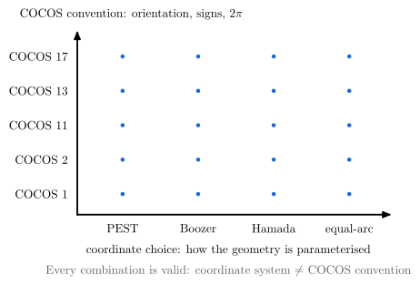
vaft.diagram.coordinates_vs_cocos()Coordinate choice and COCOS convention are independent axes, not branches of one tree.
vaft.diagram.coordinates_vs_cocos(*, labels=True)Show source vaft/diagram/_sfl_coordinates.py, lines 511–543
def coordinates_vs_cocos(*, labels: bool = True) -> Diagram:
    r"""Coordinate choice and COCOS convention are independent axes, not branches of one tree.

    Horizontal, the coordinate choice -- how the geometry is parameterised
    (PEST, Boozer, Hamada, equal-arc, all straight-field-line). Vertical,
    the COCOS convention -- orientation of the angles, signs of $\psi$, $q$,
    $B_\phi$, $I_p$ and whether $\psi$ is per radian. Every point of the grid
    is a valid, different description of the same equilibrium: changing one
    axis does not change the other (Sauter and Medvedev 2013).
    """
    labels = _check_labels(labels)
    dx, dy = 2.2, 1.0
    items: List = [Arrow((0.0, 0.0), (dx * len(_COORDINATE_AXIS) + 0.4, 0.0), "chart axis", role="axes"),
                   Arrow((0.0, 0.0), (0.0, dy * len(_COCOS_AXIS) + 0.4), "chart axis", role="axes")]
    for i, name in enumerate(_COORDINATE_AXIS):
        for j, cocos in enumerate(_COCOS_AXIS):
            items.append(Marker((dx * (i + 0.6), dy * (j + 0.6)), "o", "opoint", role=f"combination:{name}:{cocos}"))
        if labels:
            items.append(Label((dx * (i + 0.6), -0.15), name, "small label", anchor="north", role="coordinate_axis"))
    if labels:
        for j, cocos in enumerate(_COCOS_AXIS):
            items.append(Label((-0.15, dy * (j + 0.6)), f"COCOS {cocos}", "small label", anchor="east",
                               role="cocos_axis"))
        items += [Label((dx * len(_COORDINATE_AXIS) / 2, -0.75),
                        "coordinate choice: how the geometry is parameterised", "small label", anchor="north",
                        role="coordinate_axis"),
                  Label((-1.8, dy * len(_COCOS_AXIS) + 0.55),
                        "COCOS convention: orientation, signs, $2\\pi$", "small label", anchor="south west",
                        role="cocos_axis"),
                  Label((dx * len(_COORDINATE_AXIS) / 2, -1.35), "Every combination is valid: coordinate system "
                        "$\\neq$ COCOS convention", "note", anchor="north", role="note")]
    return Diagram("coordinates_vs_cocos", Scene(tuple(items)),
                   model={"coordinates": _COORDINATE_AXIS, "cocos": _COCOS_AXIS})
Formats .svg .tex .pdf the SVG above is committed; build the others locally
import vaft.diagram

d = vaft.diagram.coordinates_vs_cocos()
d.tikz  # the TikZ document as text
d.save("coordinates_vs_cocos.svg")  # rendered vector image, the canonical artifact; needs latex, dvisvgm
d.save("coordinates_vs_cocos.tex")  # the complete TikZ document, the text source
d.save("coordinates_vs_cocos.pdf")  # vector PDF; needs pdflatex
Clebsch labels, field-aligned and ballooning representations
Module vaft.diagram._ballooning
clebsch_field_line_label
1 asset
source
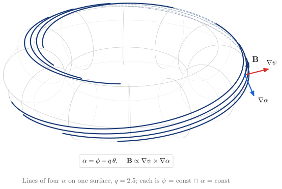
vaft.diagram.clebsch_field_line_label()A field line is where $\psi$ = const meets $\alpha$ = const.
vaft.diagram.clebsch_field_line_label(q=2.5, *, labels=True)Show source vaft/diagram/_ballooning.py, lines 71–141
def clebsch_field_line_label(q: float = 2.5, *, labels: bool = True) -> Diagram:
    r"""A field line is where $\psi$ = const meets $\alpha$ = const.

    On one flux surface (safety factor ``q``), field lines of several
    labels $\alpha = \phi - q\theta$ (``field_line_label``), each followed
    over one toroidal transit. At a point of one line the two gradients --
    $\nabla\psi$ normal to the surface, $\nabla\alpha$ in it across the lines
    -- and $\mathbf B \propto \nabla\psi\times\nabla\alpha$ along the line. That
    order holds for ``helical_phase``'s angles ($\theta$ counter-clockwise from
    the outboard midplane, $\phi$ counter-clockwise from above, so
    $(\psi, \theta, \phi)$ is left-handed) with $\psi$ rising outward and
    $\mathbf B$ along $+\phi$, $+\theta$; in right-handed coordinates (e.g.
    $\theta$ clockwise) it is $\nabla\alpha\times\nabla\psi$, the
    Connor--Hastie--Taylor form.
    """
    try:
        q = float(q)
    except (TypeError, ValueError):
        raise ValueError(f"q must be a number, not {q!r}") from None
    if not (math.isfinite(q) and 1.0 <= q <= 5.0):
        raise ValueError(f"q must lie in [1, 5], not {q!r}")
    labels = _check_labels(labels)
    items: List = _torus_wireframe()
    phi_cut = _camera_cut()
    alphas = [phi_cut + 0.5 * math.pi + k * 0.5 for k in range(4)]
    lines = {}
    theta = np.linspace(-0.5 * math.pi / q, 1.5 * math.pi / q, 600)  # one toroidal transit, centred near the front
    for k, a in enumerate(alphas):
        phi = a + q * theta
        pts = _torus(_A, theta, phi)
        lines[k] = {"alpha": a, "points": pts, "label": field_line_label(phi, theta, q)}
        items += _split_line(pts, theta, phi, role=f"field_line:{k}")
    # at a visible point of the second line: grad psi, grad alpha and their cross product
    k0 = 1
    th0 = 0.35
    ph0 = alphas[k0] + q * th0
    P = _torus(_A, th0, ph0)
    n_hat = _torus_normal(np.array(th0), np.array(ph0))
    R = _R0 + _A * math.cos(th0)
    e_theta = np.array([-math.sin(th0) * math.cos(ph0), -math.sin(th0) * math.sin(ph0), math.cos(th0)])
    e_phi = np.array([-math.sin(ph0), math.cos(ph0), 0.0])
    grad_alpha = e_phi / R - q * e_theta / _A  # grad(phi - q theta), with theta the geometric angle here
    b_dir = np.cross(n_hat, grad_alpha)  # B ~ grad(psi) x grad(alpha): along +phi, +theta with psi rising outward
    tangent = (_torus(_A, th0 + 1e-4, ph0 + q * 1e-4) - P)
    L = 0.9
    items += [
        Arrow(tuple(_p3(P)), tuple(_p3(P + L * n_hat)), "drift", role="grad_psi"),
        Arrow(tuple(_p3(P)), tuple(_p3(P + L * grad_alpha / np.linalg.norm(grad_alpha))), "drift ion",
              role="grad_alpha"),
        Arrow(tuple(_p3(P)), tuple(_p3(P + L * b_dir / np.linalg.norm(b_dir))), "field vector", role="B"),
        Marker(tuple(_p3(P)), "o", "opoint", role="B"),
    ]
    if labels:
        items += [
            Label(tuple(_p3(P + 1.05 * L * n_hat)), "$\\nabla\\psi$", "small label", anchor="south", role="grad_psi"),
            Label(tuple(_p3(P + 1.1 * L * grad_alpha / np.linalg.norm(grad_alpha))), "$\\nabla\\alpha$",
                  "small label", anchor="west", role="grad_alpha"),
            Label(tuple(_p3(P + 1.1 * L * b_dir / np.linalg.norm(b_dir))), "$\\mathbf{B}$", "label", anchor="west",
                  role="B"),
        ]
        y_box = _below(items) - 0.2
        items += [
            Label((float(_p3(np.zeros(3))[0]), y_box),
                  f"$\\displaystyle {formula_equation(field_line_label)}$, $\\quad\\mathbf{{B}} \\propto \\nabla\\psi\\times\\nabla\\alpha$",
                  "formula box", anchor="north", role="equations"),
            _note(f"Lines of four $\\alpha$ on one surface, $q = {q:g}$; each is $\\psi$ = const "
                  "$\\cap$ $\\alpha$ = const", float(_p3(np.zeros(3))[0]), y_box - 1.1),
        ]
    model = {"q": q, "lines": lines, "point": P, "grad_alpha": grad_alpha, "normal": n_hat, "B_direction": b_dir,
             "tangent": tangent}
    return Diagram("clebsch_field_line_label", Scene(tuple(items)), model=model)
Formats .svg .tex .pdf the SVG above is committed; build the others locally
import vaft.diagram

d = vaft.diagram.clebsch_field_line_label()
d.tikz  # the TikZ document as text
d.save("clebsch_field_line_label.svg")  # rendered vector image, the canonical artifact; needs latex, dvisvgm
d.save("clebsch_field_line_label.tex")  # the complete TikZ document, the text source
d.save("clebsch_field_line_label.pdf")  # vector PDF; needs pdflatex
Formula functions referenced:
stability.field_line_label
ballooning_curvature_drive
1 asset
source
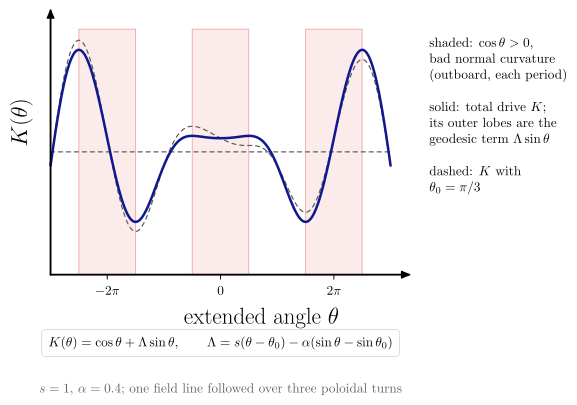
vaft.diagram.ballooning_curvature_drive()Normal curvature and the total ballooning drive along the extended angle.
vaft.diagram.ballooning_curvature_drive(*, labels=True)Show source vaft/diagram/_ballooning.py, lines 175–221
def ballooning_curvature_drive(*, labels: bool = True) -> Diagram:
    r"""Normal curvature and the total ballooning drive along the extended angle.

    Shaded: the normal curvature $\cos\theta > 0$ -- bad, on the outboard
    side, once per $2\pi$ period of the covering space. Solid: the drive
    $K = \cos\theta + \Lambda\sin\theta$ of ``s_alpha_curvature_drive`` at
    $s = 1$, $\alpha = 0.4$; beyond the first period its positive lobes come
    from the geodesic term $\Lambda\sin\theta$, which grows with $|\theta|$
    through the local shear, not from the outboard position. Dashed: the same
    drive with the ballooning angle $\theta_0 = \pi/3$.
    """
    labels = _check_labels(labels)
    s, a, th0 = _S, 0.4, math.pi / 3
    theta = np.linspace(-3.0 * math.pi, 3.0 * math.pi, 2401)
    K = s_alpha_curvature_drive(theta, s, a)
    K0 = s_alpha_curvature_drive(theta, s, a, theta0=th0)
    top = float(max(np.abs(K).max(), np.abs(K0).max()))
    chart = Chart(x_range=(float(theta[0]), float(theta[-1])), y_range=(-1.1 * top, 1.1 * top))
    chart.curves.update({"drive": np.stack([theta, K], -1), "drive_theta0": np.stack([theta, K0], -1),
                         "zero": np.array([[theta[0], 0.0], [theta[-1], 0.0]])})
    bad = _bands(theta, np.cos(theta) > 0)
    chart.parameters.update({"s": s, "alpha": a, "theta0": th0, "bad_bands": bad,
                             "drive_bands": _bands(theta, K > 0)})
    ticks = tuple(k * math.pi for k in range(-2, 3, 2))
    scene = render_chart(chart, x_label="extended angle $\\theta$", y_label="$K(\\theta)$",
                         curve_styles={"zero": "approx", "drive_theta0": "approx", "drive": "boundary"},
                         region_text={}, x_ticks=ticks, x_tick_text=("$-2\\pi$", "$0$", "$2\\pi$"))
    items: List = []
    for b0, b1 in bad:
        x0, x1 = chart.to_cm(np.array([[b0, 0.0], [b1, 0.0]]))[:, 0]
        items.append(Polyline.of([(x0, 0.0), (x1, 0.0), (x1, CHART_HEIGHT), (x0, CHART_HEIGHT)], "layer",
                                 role="bad_curvature", closed=True))
    items += list(scene.items)
    if labels:
        items += [
            Label((CHART_WIDTH + 0.9, CHART_HEIGHT - 0.1), "shaded: $\\cos\\theta > 0$,\\\\ bad normal curvature\\\\ "
                  "(outboard, each period)", "small label,align=left", anchor="north west", role="bad_curvature"),
            Label((CHART_WIDTH + 0.9, CHART_HEIGHT - 1.8), "solid: total drive $K$;\\\\ its outer lobes are the\\\\ "
                  "geodesic term $\\Lambda\\sin\\theta$", "small label,align=left", anchor="north west", role="drive"),
            Label((CHART_WIDTH + 0.9, CHART_HEIGHT - 3.5), "dashed: $K$ with\\\\ $\\theta_0 = \\pi/3$",
                  "small label,align=left", anchor="north west", role="theta0"),
            Label((CHART_WIDTH / 2, -1.45), f"$\\displaystyle {formula_equation(s_alpha_curvature_drive)}$",
                  "formula box", anchor="north", role="equations"),
            _note(f"$s = {s:g}$, $\\alpha = {a:g}$; one field line followed over three poloidal turns",
                  CHART_WIDTH / 2, -2.75),
        ]
    return Diagram("ballooning_curvature_drive", Scene(tuple(items)), model=chart)
Formats .svg .tex .pdf the SVG above is committed; build the others locally
import vaft.diagram

d = vaft.diagram.ballooning_curvature_drive()
d.tikz  # the TikZ document as text
d.save("ballooning_curvature_drive.svg")  # rendered vector image, the canonical artifact; needs latex, dvisvgm
d.save("ballooning_curvature_drive.tex")  # the complete TikZ document, the text source
d.save("ballooning_curvature_drive.pdf")  # vector PDF; needs pdflatex
Formula functions referenced:
stability.s_alpha_curvature_drive
ballooning_newcomb_test
1 asset
source
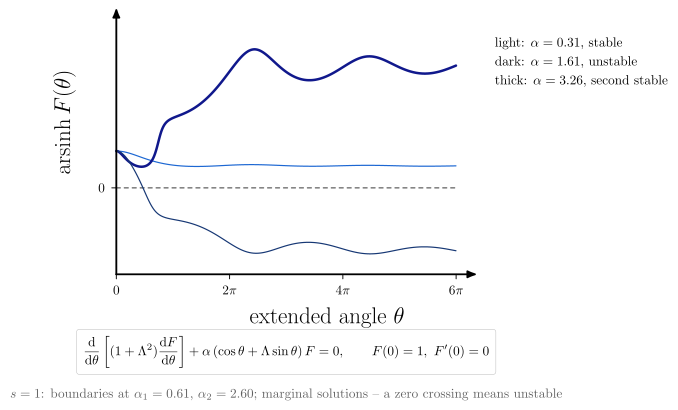
vaft.diagram.ballooning_newcomb_test()Newcomb’s test on the extended angle: stable, unstable and second stable.
vaft.diagram.ballooning_newcomb_test(*, labels=True)Show source vaft/diagram/_ballooning.py, lines 229–274
def ballooning_newcomb_test(*, labels: bool = True) -> Diagram:
    r"""Newcomb's test on the extended angle: stable, unstable and second stable.

    The even marginal ($\omega^2 = 0$) solution $F(\theta)$, $F(0) = 1$, of the
    $s$-$\alpha$ equation (``s_alpha_ballooning_solution``) at $s = 1$ for three
    pressure gradients: below the first boundary it stays positive, between
    the boundaries it crosses zero (unstable), beyond the second
    (``s_alpha_marginal_alpha``) it is positive again. These are marginal
    solutions, not localised eigenfunctions: a stable $F$ grows without
    decaying, and only the sign change carries the verdict.
    """
    labels = _check_labels(labels)
    alpha1, alpha2 = _boundaries(_S)
    cases = {"stable": 0.5 * alpha1, "unstable": 0.5 * (alpha1 + alpha2), "second_stable": 1.25 * alpha2}
    curves = {}
    for name, a in cases.items():
        theta, F = s_alpha_ballooning_solution(_S, a, theta_max=6.0 * math.pi)
        # arsinh keeps the sign -- the zero crossing is the verdict -- and compresses the growth
        curves[name] = np.stack([theta, np.arcsinh(F)], -1)
    lo = min(float(c[:, 1].min()) for c in curves.values())
    hi = max(float(c[:, 1].max()) for c in curves.values())
    chart = Chart(x_range=(0.0, 6.0 * math.pi), y_range=(min(lo, 0.0) - 0.1 * (hi - lo), hi + 0.1 * (hi - lo)))
    chart.curves.update(curves)
    chart.curves["zero"] = np.array([[0.0, 0.0], [6.0 * math.pi, 0.0]])
    chart.parameters.update({"s": _S, "alpha": cases, "alpha1": alpha1, "alpha2": alpha2})
    scene = render_chart(chart, x_label="extended angle $\\theta$", y_label="$\\mathrm{arsinh}\\,F(\\theta)$",
                         curve_styles={"zero": "approx", "stable": "orbit ion", "second_stable": "boundary",
                                       "unstable": "orbit electron"},
                         region_text={}, x_ticks=(0.0, 2 * math.pi, 4 * math.pi, 6 * math.pi),
                         x_tick_text=("$0$", "$2\\pi$", "$4\\pi$", "$6\\pi$"), y_ticks=(0.0,))
    items: List = []
    if labels:
        items += [
            Label((CHART_WIDTH + 0.9, CHART_HEIGHT - 0.1), f"light: $\\alpha = {cases['stable']:.2f}$, stable",
                  "small label", anchor="north west", role="stable"),
            Label((CHART_WIDTH + 0.9, CHART_HEIGHT - 0.6), f"dark: $\\alpha = {cases['unstable']:.2f}$, unstable",
                  "small label", anchor="north west", role="unstable"),
            Label((CHART_WIDTH + 0.9, CHART_HEIGHT - 1.1),
                  f"thick: $\\alpha = {cases['second_stable']:.2f}$, second stable", "small label",
                  anchor="north west", role="second_stable"),
            Label((CHART_WIDTH / 2, -1.45), f"$\\displaystyle {formula_equation(s_alpha_ballooning_solution)}$",
                  "formula box", anchor="north", role="equations"),
            _note(f"$s = {_S:g}$: boundaries at $\\alpha_1 = {alpha1:.2f}$, $\\alpha_2 = {alpha2:.2f}$; marginal "
                  "solutions -- a zero crossing means unstable", CHART_WIDTH / 2, -2.9),
        ]
    return Diagram("ballooning_newcomb_test", scene + Scene(tuple(items)), model=chart)
Formats .svg .tex .pdf the SVG above is committed; build the others locally
import vaft.diagram

d = vaft.diagram.ballooning_newcomb_test()
d.tikz  # the TikZ document as text
d.save("ballooning_newcomb_test.svg")  # rendered vector image, the canonical artifact; needs latex, dvisvgm
d.save("ballooning_newcomb_test.tex")  # the complete TikZ document, the text source
d.save("ballooning_newcomb_test.pdf")  # vector PDF; needs pdflatex
Formula functions referenced:
stability.s_alpha_ballooning_solution, stability.s_alpha_marginal_alpha
ballooning_harmonic_envelope
1 asset
source
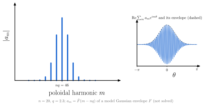
vaft.diagram.ballooning_harmonic_envelope()A ballooning mode is many coupled harmonics $m \approx nq$ under one envelope.
vaft.diagram.ballooning_harmonic_envelope(n=20, *, labels=True)Show source vaft/diagram/_ballooning.py, lines 285–333
def ballooning_harmonic_envelope(n: int = 20, *, labels: bool = True) -> Diagram:
    r"""A ballooning mode is many coupled harmonics $m \approx nq$ under one envelope.

    The ballooning transform writes the poloidal harmonics on a surface as
    $a_m = \hat F(m - nq)$, the Fourier transform of the envelope $F$ on the
    extended angle. With a model envelope localised at the outboard midplane
    (a Gaussian of width 0.8 rad, stated, not solved), the bars are $|a_m|$
    for toroidal mode number $n$ and $q = 2.3$. Right: their sum
    $\mathrm{Re}\sum_m a_m e^{im\theta}$ -- fast oscillation at $m \approx nq$
    whose amplitude follows the envelope, the ballooning structure.
    """
    if isinstance(n, bool) or not isinstance(n, (int, np.integer)) or not 5 <= n <= 60:
        raise ValueError(f"n must be an integer from 5 to 60, not {n!r}")
    labels = _check_labels(labels)
    q = 2.3
    eta = np.linspace(-4.0 * math.pi, 4.0 * math.pi, 8001)
    env = np.exp(-0.5 * (eta / _ENVELOPE_WIDTH) ** 2)
    m0 = n * q
    m = np.arange(int(m0) - 8, int(m0) + 10)
    amps = np.array([np.trapezoid(env * np.exp(-1j * (mm - m0) * eta), eta).real for mm in m]) / (2.0 * math.pi)
    grid = np.linspace(-math.pi, math.pi, 2401)
    field = np.real(sum(a * np.exp(1j * mm * grid) for a, mm in zip(amps, m)))
    field = field / np.max(np.abs(field))
    # left: the spectrum
    chart = Chart(x_range=(float(m[0]) - 0.5, float(m[-1]) + 0.5), y_range=(0.0, 1.15 * float(np.abs(amps).max())))
    for mm, a in zip(m, amps):
        chart.curves[f"bar_{mm}"] = np.array([[mm, 0.0], [mm, abs(a)]])
    chart.parameters.update({"n": n, "q": q, "m": m, "amplitudes": amps, "envelope_width": _ENVELOPE_WIDTH})
    scene = render_chart(chart, x_label="poloidal harmonic $m$", y_label="$|a_m|$",
                         curve_styles={f"bar_{mm}": "component imag" for mm in m}, region_text={},
                         x_ticks=(float(round(m0)),), x_tick_text=(f"$nq = {m0:g}$",))
    items: List = [Polyline(it.points, it.style, "harmonic", it.closed) if isinstance(it, Polyline)
                   and it.role.startswith("bar_") else it for it in scene.items]
    right = Chart(x_range=(-math.pi, math.pi), y_range=(-1.1, 1.1))
    right.curves["field"] = np.stack([grid, field], -1)
    right.curves["envelope"] = np.stack([grid, np.exp(-0.5 * (grid / _ENVELOPE_WIDTH) ** 2)], -1)
    sub = render_chart(right, x_label="$\\theta$", y_label="", curve_styles={"envelope": "approx", "field": "orbit ion"},
                       region_text={}, x_ticks=(-math.pi, 0.0, math.pi), x_tick_text=("$-\\pi$", "$0$", "$\\pi$"))
    items += list(sub.transformed(scale=0.6, offset=(CHART_WIDTH + 2.0, 0.2 * CHART_HEIGHT)).items)
    if labels:
        items += [
            Label((CHART_WIDTH + 2.0 + 0.3 * CHART_WIDTH, 0.2 * CHART_HEIGHT + 0.62 * CHART_HEIGHT),
                  "$\\mathrm{Re}\\sum_m a_m e^{im\\theta}$ and its envelope (dashed)", "small label", anchor="south",
                  role="field"),
            _note(f"$n = {n}$, $q = {q:g}$; $a_m = \\hat F(m - nq)$ of a model Gaussian envelope $F$ (not solved)",
                  0.5 * (CHART_WIDTH + 2.0 + 0.6 * CHART_WIDTH), -1.5),
        ]
    chart.parameters["field"] = np.stack([grid, field], -1)
    return Diagram("ballooning_harmonic_envelope", Scene(tuple(items)), model=chart)
Formats .svg .tex .pdf the SVG above is committed; build the others locally
import vaft.diagram

d = vaft.diagram.ballooning_harmonic_envelope()
d.tikz  # the TikZ document as text
d.save("ballooning_harmonic_envelope.svg")  # rendered vector image, the canonical artifact; needs latex, dvisvgm
d.save("ballooning_harmonic_envelope.tex")  # the complete TikZ document, the text source
d.save("ballooning_harmonic_envelope.pdf")  # vector PDF; needs pdflatex
ballooning_workflow
1 asset
source
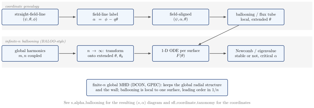
vaft.diagram.ballooning_workflow()From global harmonics to the infinite-$n$ ballooning equation, and the coordinate genealogy.
vaft.diagram.ballooning_workflow(*, labels=True)Show source vaft/diagram/_ballooning.py, lines 341–376
def ballooning_workflow(*, labels: bool = True) -> Diagram:
    r"""From global harmonics to the infinite-$n$ ballooning equation, and the coordinate genealogy.

    Top row: the coordinate hierarchy -- straight-field-line coordinates,
    the field-line label, field-aligned coordinates, ballooning / flux-tube
    representations. Middle: the BALOO-style path -- high-$n$ ordering, the
    ballooning transform onto the extended angle, one 1-D equation per
    surface, a Newcomb or eigenvalue test, an $(s, \alpha)$ verdict. Bottom:
    what a finite-$n$ global calculation keeps that it drops.
    """
    labels = _check_labels(labels)
    W, H = 4.0, 1.35
    items: List = []
    items += band(-1.0, 25.4, 2.0, 4.4, "coordinate genealogy", role="band:coordinates")
    items += band(-1.0, 25.4, -1.2, 1.45, "infinite-$n$ ballooning (BALOO-style)", role="band:ballooning")
    top = [("sfl", "straight-field-line\\\\ $(\\psi, \\theta, \\phi)$"), ("label", "field-line label\\\\ $\\alpha = \\phi - q\\theta$"),
           ("aligned", "field-aligned\\\\ $(\\psi, \\alpha, \\theta)$"), ("tube", "ballooning / flux tube\\\\ local, extended $\\theta$")]
    mid = [("global", "global harmonics\\\\ $m, n$ coupled"), ("transform", "$n \\to \\infty$: transform\\\\ onto extended $\\theta$, $\\theta_0$"),
           ("ode", "1-D ODE per surface\\\\ $F(\\theta)$"), ("test", "Newcomb / eigenvalue\\\\ stable or not, critical $\\alpha$")]
    nodes = {}
    for row, y in ((top, 3.1), (mid, 0.0)):
        for i, (key, text) in enumerate(row):
            b = box(1.4 + 6.4 * i, y, W + 0.8, H, text, role=f"node:{key}", latex=True)
            nodes[key] = b
            items += list(b.items)
        for (k1, _), (k2, _) in zip(row, row[1:]):
            items.append(connector(nodes[k1], nodes[k2], role=f"edge:{k1}->{k2}"))
    items.append(connector(nodes["tube"], nodes["ode"], role="edge:tube->ode"))
    glob = box(12.2, -2.9, 12.0, 1.4, "finite-$n$ global MHD (DCON, GPEC): keeps the global radial structure and the wall; "
               "ballooning is local to one surface, leading order in $1/n$", role="node:global_mhd", latex=True)
    items += list(glob.items)
    if labels:
        items.append(_note("See s\\_alpha\\_ballooning for the resulting $(s, \\alpha)$ diagram and "
                           "sfl\\_coordinate\\_taxonomy for the coordinates", 12.2, -3.9))
    model = {"nodes": tuple(nodes)}
    return Diagram("ballooning_workflow", Scene(tuple(items)), model=model)
Formats .svg .tex .pdf the SVG above is committed; build the others locally
import vaft.diagram

d = vaft.diagram.ballooning_workflow()
d.tikz  # the TikZ document as text
d.save("ballooning_workflow.svg")  # rendered vector image, the canonical artifact; needs latex, dvisvgm
d.save("ballooning_workflow.tex")  # the complete TikZ document, the text source
d.save("ballooning_workflow.pdf")  # vector PDF; needs pdflatex
Slab resonant layers: tearing and twisting parity, harmonic coupling
Module vaft.diagram._slab_parity
slab_parity
2 assets
source
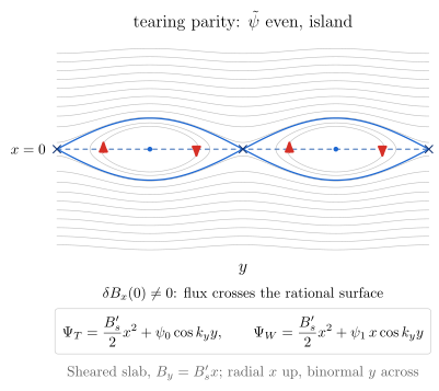
vaft.diagram.slab_parity(parity='tearing')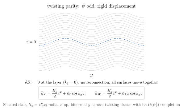
vaft.diagram.slab_parity(parity='twisting')Tearing or twisting parity at a rational surface, as contours of the helical flux.
vaft.diagram.slab_parity(parity='tearing', *, labels=True)Show source vaft/diagram/_slab_parity.py, lines 130–154
def slab_parity(parity: str = "tearing", *, labels: bool = True) -> Diagram:
    r"""Tearing or twisting parity at a rational surface, as contours of the helical flux.

    Contours of $\Psi$ from ``slab_perturbed_flux`` over two wavelengths: for
    tearing parity the island of width $4\sqrt{\psi_0/B_s'}$ with its O- and
    X-points and separatrix, and $\delta B_x \ne 0$ on $x = 0$ (arrows); for
    twisting parity $\Psi_W$ completed with its $O(\psi_1^2)$ term, so every
    surface -- the rational one included -- is displaced together by
    $\xi = -\psi_1\cos k_yy/B_s'$, with no normal field at the layer and no
    reconnection.
    """
    if parity not in PARITIES:
        raise ValueError(f"parity must be one of {PARITIES}, not {parity!r}")
    labels = _check_labels(labels)
    panel = _panel(parity, labels)
    items = list(panel["items"])
    if labels:
        items += [
            Label((0.5 * _W, -0.5 * _H - 1.35), f"$\\displaystyle {formula_equation(slab_perturbed_flux)}$",
                  "formula box", anchor="north", role="equations"),
            Label((0.5 * _W, -0.5 * _H - 2.6), "Sheared slab, $B_y = B_s'x$; radial $x$ up, binormal $y$ across"
                  + ("; twisting drawn with its $O(\\psi_1^2)$ completion" if parity == "twisting" else ""),
                  "note", anchor="north", role="note"),
        ]
    return Diagram(f"slab_parity_{parity}", Scene(tuple(items)), model={"parity": parity, **panel["info"]})
Formats .svg .tex .pdf the SVG above is committed; build the others locally
import vaft.diagram

d = vaft.diagram.slab_parity(parity='tearing')
d.tikz  # the TikZ document as text
d.save("slab_parity_tearing.svg")  # rendered vector image, the canonical artifact; needs latex, dvisvgm
d.save("slab_parity_tearing.tex")  # the complete TikZ document, the text source
d.save("slab_parity_tearing.pdf")  # vector PDF; needs pdflatex
Formula functions referenced:
stability.slab_perturbed_flux
slab_parity_comparison
1 asset
source
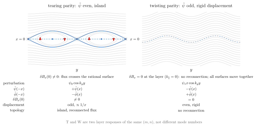
vaft.diagram.slab_parity_comparison()Tearing and twisting parity side by side, with what tells them apart.
vaft.diagram.slab_parity_comparison(*, labels=True)Show source vaft/diagram/_slab_parity.py, lines 157–188
def slab_parity_comparison(*, labels: bool = True) -> Diagram:
    r"""Tearing and twisting parity side by side, with what tells them apart.

    The two panels of ``slab_parity``, and under them the defining
    properties: the parity of $\tilde\psi$ and of the stream function, the
    normal field on the rational surface, and whether flux reconnects. The
    parity is a property of the local layer response; the harmonic index $m$
    of ``poloidal_harmonic_coupling`` is a different index.
    """
    labels = _check_labels(labels)
    items: List = []
    info = {}
    for i, parity in enumerate(PARITIES):
        panel = _panel(parity, labels, x_off=i * (_W + 1.5))
        items += panel["items"]
        info[parity] = panel["info"]
    if labels:
        rows = [("perturbation", "$\\psi_0\\cos k_yy$", "$\\psi_1x\\cos k_yy$"),
                ("$\\tilde\\psi(-x)$", "$+\\tilde\\psi(x)$", "$-\\tilde\\psi(x)$"),
                ("$\\tilde\\phi(-x)$", "$-\\tilde\\phi(x)$", "$+\\tilde\\phi(x)$"),
                ("$\\delta B_x(0)$", "$\\ne 0$", "$= 0$"),
                ("displacement", "odd, $\\propto 1/x$", "even, rigid"),
                ("topology", "island, reconnected flux", "no reconnection")]
        y0 = -0.5 * _H - 1.6
        for j, (name, t, w) in enumerate(rows):
            y = y0 - 0.5 * j
            items += [Label((-0.2, y), name, "small label", anchor="east", role="table"),
                      Label((0.5 * _W, y), t, "small label", anchor="center", role="table"),
                      Label((_W + 1.5 + 0.5 * _W, y), w, "small label", anchor="center", role="table")]
        items.append(Label((_W + 0.75, y0 - 3.3), "T and W are two layer responses of the same $(m, n)$, not "
                           "different mode numbers", "note", anchor="north", role="note"))
    return Diagram("slab_parity_comparison", Scene(tuple(items)), model=info)
Formats .svg .tex .pdf the SVG above is committed; build the others locally
import vaft.diagram

d = vaft.diagram.slab_parity_comparison()
d.tikz  # the TikZ document as text
d.save("slab_parity_comparison.svg")  # rendered vector image, the canonical artifact; needs latex, dvisvgm
d.save("slab_parity_comparison.tex")  # the complete TikZ document, the text source
d.save("slab_parity_comparison.pdf")  # vector PDF; needs pdflatex
Formula functions referenced:
stability.slab_perturbed_flux
poloidal_harmonic_coupling
1 asset
source
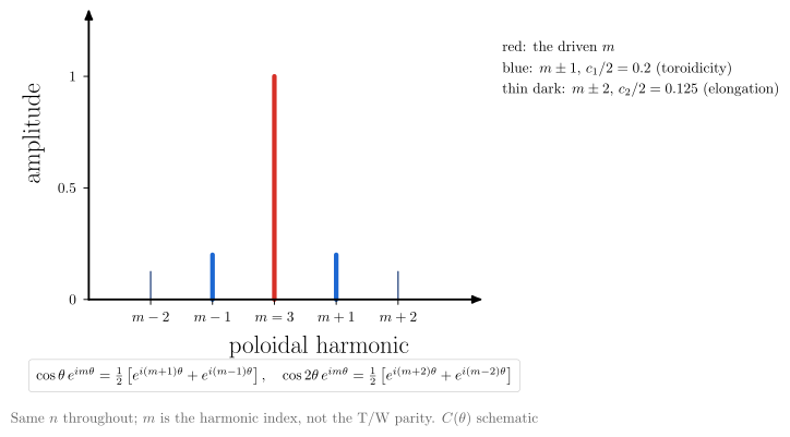
vaft.diagram.poloidal_harmonic_coupling()Toroidicity couples $m$ to $m \pm 1$, elongation to $m \pm 2$, at fixed $n$.
vaft.diagram.poloidal_harmonic_coupling(m=3, *, labels=True)Show source vaft/diagram/_slab_parity.py, lines 205–248
def poloidal_harmonic_coupling(m: int = 3, *, labels: bool = True) -> Diagram:
    r"""Toroidicity couples $m$ to $m \pm 1$, elongation to $m \pm 2$, at fixed $n$.

    A single harmonic $e^{im\theta}$ multiplied by an equilibrium coefficient
    $C(\theta) = 1 + c_1\cos\theta + c_2\cos 2\theta$ (schematic $c_1 = 0.4$ for
    toroidicity and the Shafranov shift, $c_2 = 0.25$ for elongation) has the
    spectrum below, computed by FFT: $\cos\theta\,e^{im\theta} =
    \tfrac12[e^{i(m+1)\theta} + e^{i(m-1)\theta}]$, and $\cos 2\theta$ likewise
    with $m \pm 2$. Real shaped equilibria have more harmonics and couple more.
    """
    if isinstance(m, bool) or not isinstance(m, (int, np.integer)) or not 1 <= m <= 12:
        raise ValueError(f"m must be an integer from 1 to 12, not {m!r}")
    labels = _check_labels(labels)
    c1, c2 = 0.4, 0.25
    spectrum = harmonic_coupling_spectrum(m, c1, c2)
    ms = sorted(spectrum)
    chart = Chart(x_range=(m - 3.0, m + 3.0), y_range=(0.0, 1.2))
    source = {m: "self", m - 1: "cos1", m + 1: "cos1", m - 2: "cos2", m + 2: "cos2"}
    style = {"self": "component real", "cos1": "component imag", "cos2": "orbit electron"}
    for k in ms:
        chart.curves[f"bar_{k}"] = np.array([[k, 0.0], [k, abs(spectrum[k])]])
    chart.parameters.update({"m": m, "c1": c1, "c2": c2, "spectrum": spectrum})
    ticks = tuple(float(k) for k in range(m - 2, m + 3))
    tick_text = ("$m-2$", "$m-1$", f"$m = {m}$", "$m+1$", "$m+2$")
    scene = render_chart(chart, x_label="poloidal harmonic", y_label="amplitude",
                         curve_styles={f"bar_{k}": style[source[k]] for k in ms}, region_text={},
                         x_ticks=ticks, x_tick_text=tick_text, y_ticks=(0.0, 0.5, 1.0))
    items = [Polyline(it.points, it.style, f"harmonic:{source[int(it.role.split('_')[1])]}", it.closed)
             if isinstance(it, Polyline) and it.role.startswith("bar_") else it for it in scene.items]
    if labels:
        items += [
            Label((CHART_WIDTH + 0.9, CHART_HEIGHT - 0.1), "red: the driven $m$", "small label", anchor="north west",
                  role="legend"),
            Label((CHART_WIDTH + 0.9, CHART_HEIGHT - 0.6), f"blue: $m \\pm 1$, $c_1/2 = {c1 / 2:g}$ (toroidicity)",
                  "small label", anchor="north west", role="legend"),
            Label((CHART_WIDTH + 0.9, CHART_HEIGHT - 1.1), f"thin dark: $m \\pm 2$, $c_2/2 = {c2 / 2:g}$ (elongation)",
                  "small label", anchor="north west", role="legend"),
            Label((CHART_WIDTH / 2, -1.45), "$\\cos\\theta\\,e^{im\\theta} = \\tfrac12\\left[e^{i(m+1)\\theta} + "
                  "e^{i(m-1)\\theta}\\right],\\quad \\cos 2\\theta\\,e^{im\\theta} = \\tfrac12\\left[e^{i(m+2)\\theta} + "
                  "e^{i(m-2)\\theta}\\right]$", "formula box", anchor="north", role="equations"),
            Label((CHART_WIDTH / 2, -2.6), "Same $n$ throughout; $m$ is the harmonic index, not the T/W parity. "
                  "$C(\\theta)$ schematic", "note", anchor="north", role="note"),
        ]
    return Diagram("poloidal_harmonic_coupling", Scene(tuple(items)), model=chart)
Formats .svg .tex .pdf the SVG above is committed; build the others locally
import vaft.diagram

d = vaft.diagram.poloidal_harmonic_coupling()
d.tikz  # the TikZ document as text
d.save("poloidal_harmonic_coupling.svg")  # rendered vector image, the canonical artifact; needs latex, dvisvgm
d.save("poloidal_harmonic_coupling.tex")  # the complete TikZ document, the text source
d.save("poloidal_harmonic_coupling.pdf")  # vector PDF; needs pdflatex
resonant_layer_matching
1 asset
source
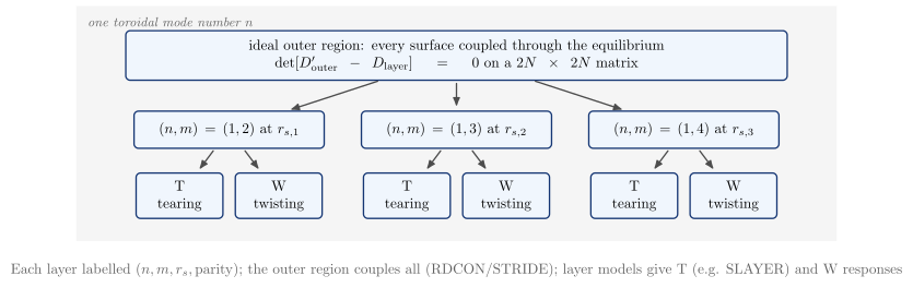
vaft.diagram.resonant_layer_matching()Several rational surfaces, each with a tearing and a twisting channel, matched through the outer region.
vaft.diagram.resonant_layer_matching(*, labels=True)Show source vaft/diagram/_slab_parity.py, lines 256–288
def resonant_layer_matching(*, labels: bool = True) -> Diagram:
    r"""Several rational surfaces, each with a tearing and a twisting channel, matched through the outer region.

    For one $n$, rational surfaces $q = m/n$ ($m = 2, 3, 4$ at $n = 1$) each
    carry a tearing-parity (T) and a twisting-parity (W) layer response. The
    ideal outer region couples all of them -- through the poloidal-harmonic
    coupling of the equilibrium -- into one $2N \times 2N$ matching matrix
    (the multi-surface generalisation of $\Delta'$ that RDCON/STRIDE compute),
    while the layer physics is solved surface by surface (SLAYER-type models
    for the tearing response).
    """
    labels = _check_labels(labels)
    items: List = []
    items += band(-1.2, 17.2, -4.1, 1.6, "one toroidal mode number $n$", role="band")
    outer = box(8.0, 0.4, 16.0, 1.2, "ideal outer region: every surface coupled through the equilibrium"
                "\\\\ $\\det[D'_\\mathrm{outer} - D_\\mathrm{layer}] = 0$ on a $2N\\times2N$ matrix", role="outer",
                latex=True)
    items += list(outer.items)
    surfaces = []
    for i, m in enumerate((2, 3, 4)):
        x = 2.5 + 5.5 * i
        head = box(x, -1.4, 4.6, 0.9, f"$(n, m) = (1, {m})$ at $r_{{s,{i + 1}}}$", role=f"surface:{m}", latex=True)
        t = box(x - 1.2, -3.0, 2.1, 1.1, "T\\\\ tearing", role=f"layer:{m}:tearing", latex=True)
        w = box(x + 1.2, -3.0, 2.1, 1.1, "W\\\\ twisting", role=f"layer:{m}:twisting", latex=True)
        items += list(head.items) + list(t.items) + list(w.items)
        items += [connector(outer, head, role=f"edge:outer->{m}"), connector(head, t, role=f"edge:{m}->T"),
                  connector(head, w, role=f"edge:{m}->W")]
        surfaces.append(m)
    if labels:
        items.append(Label((8.0, -4.5), "Each layer labelled $(n, m, r_s, \\mathrm{parity})$; the outer region couples "
                           "all (RDCON/STRIDE); layer models give T (e.g. SLAYER) and W responses", "note",
                           anchor="north", role="note"))
    return Diagram("resonant_layer_matching", Scene(tuple(items)), model={"surfaces": tuple(surfaces)})
Formats .svg .tex .pdf the SVG above is committed; build the others locally
import vaft.diagram

d = vaft.diagram.resonant_layer_matching()
d.tikz  # the TikZ document as text
d.save("resonant_layer_matching.svg")  # rendered vector image, the canonical artifact; needs latex, dvisvgm
d.save("resonant_layer_matching.tex")  # the complete TikZ document, the text source
d.save("resonant_layer_matching.pdf")  # vector PDF; needs pdflatex
Disruption physics: the quench sequence, its causal chain, runaway generation and energy paths
Module vaft.diagram._disruption
disruption_timeline
1 asset
source
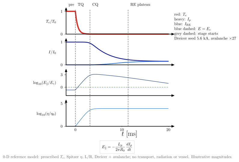
vaft.diagram.disruption_timeline()A disruption on one time axis, from a 0-D reference model built of the formulas.
vaft.diagram.disruption_timeline(*, labels=True)Show source vaft/diagram/_disruption.py, lines 130–208
def disruption_timeline(*, labels: bool = True) -> Diagram:
    r"""A disruption on one time axis, from a 0-D reference model built of the formulas.

    Four stacked panels over $-2$ to $20$ ms: the prescribed thermal quench
    $T_e/T_0$ (``thermal_quench_temperature``, 2 keV to 5 eV in 0.5 ms);
    the plasma and runaway currents; $\log_{10}(E_\parallel/E_c)$ with $E_c$
    from ``connor_hastie_critical_field``; and the resistivity
    (``spitzer_resistivity_from_T_e_Z_eff_ln_Lambda``). The current decays by
    L/R with $R_p$ rising as the plasma cools, the induced field reaches about
    $10^3E_c$ (and $E/E_D \approx 2\,\%$), a Dreicer seed of a few kA forms
    and the avalanche multiplies it a few e-folds -- at 1 MA only a few; at
    reactor currents tens -- until a runaway plateau carries part of the
    current (``reference_model``; $R_0 = 1.7$ m, $a = 0.5$ m, 1 MA,
    $5\times10^{19}$ m$^{-3}$). Illustrative magnitudes, not to scale for any
    machine: no universal waveform or timescale is implied.
    """
    labels = _check_labels(labels)
    m = reference_model()
    p = m["params"]
    t_ms = m["t"] * 1e3
    panels = [
        ("T_e", "$T_e/T_0$", m["T_e"] / p["T_0"], (0.0, 1.1), "component real"),
        ("I", "$I/I_0$", None, (0.0, 1.1), None),
        ("E", "$\\log_{10}(E_\\parallel/E_c)$", np.log10(np.maximum(m["E"] / m["E_c"], 1e-3)), (-2.0, 4.0),
         "orbit electron"),
        ("eta", "$\\log_{10}(\\eta/\\eta_0)$", np.log10(m["eta"] / m["eta"][0]), (0.0, 5.5), "orbit ion"),
    ]
    height = 2.2
    items: List = []
    edges = _phase_edges(m)
    x_range = (float(t_ms[0]), float(t_ms[-1]))
    for k, (key, ylabel, y, y_range, style) in enumerate(panels):
        chart = Chart(x_range=x_range, y_range=y_range)
        if key == "I":
            chart.curves["I_p"] = np.stack([t_ms, m["I_p"] / p["I_0"]], -1)
            chart.curves["I_RE"] = np.stack([t_ms, m["I_RE"] / p["I_0"]], -1)
            styles = {"I_p": "boundary", "I_RE": "crest"}
        else:
            chart.curves[key] = np.stack([t_ms, y], -1)
            styles = {key: style}
        if key == "E":
            chart.curves["E_c"] = np.array([[x_range[0], 0.0], [x_range[1], 0.0]])
            styles["E_c"] = "rational"
        y_ticks = {"E": (0.0, 3.0), "eta": (0.0, 5.0), "T_e": (0.0, 1.0), "I": (0.0, 1.0)}[key]
        scene = render_chart(chart, x_label="$t$ [ms]" if k == len(panels) - 1 else "", y_label="",
                             curve_styles=styles, region_text={},
                             x_ticks=(0.0, 10.0, 20.0) if k == len(panels) - 1 else (), y_ticks=y_ticks,
                             y_tick_text=tuple(f"${v:g}$" for v in y_ticks))
        offset = (0.0, (len(panels) - 1 - k) * (height + 0.5))
        items += _squash(scene, height / CHART_HEIGHT, offset)
        if labels:
            items.append(Label((-0.75, offset[1] + 0.5 * height), ylabel, "small label", anchor="east",
                               role=f"panel:{key}"))
    total_h = len(panels) * (height + 0.5) - 0.5
    # stage boundaries across all panels
    chart0 = Chart(x_range=x_range, y_range=(0.0, 1.0))
    for name, t0 in edges.items():
        x = float(chart0.to_cm(np.array([t0 * 1e3, 0.0]))[0])
        items.append(Polyline.of([(x, 0.0), (x, total_h)], "approx", role=f"stage:{name}"))
        if labels:
            text = {"thermal_quench": "TQ", "current_quench": "CQ", "re_plateau": "RE plateau"}[name]
            items.append(Label((x + 0.08, total_h + 0.1), text, "small label", anchor="south west",
                               role=f"stage:{name}"))
    if labels:
        items += [
            Label((0.1, total_h + 0.1), "pre", "small label", anchor="south west", role="stage:pre"),
            Label((CHART_WIDTH + 0.4, total_h - 0.2), "red: $T_e$\\\\ heavy: $I_p$\\\\ blue: $I_\\mathrm{RE}$\\\\ "
                  "blue dashed: $E = E_c$\\\\ grey dashed: stage starts\\\\ "
                  f"Dreicer seed {m['seed_current'] / 1e3:.1f} kA, avalanche $\\times{m['avalanche_gain']:.0f}$",
                  "small label,align=left", anchor="north west", role="legend"),
            Label((CHART_WIDTH / 2, -1.25), f"$\\displaystyle {formula_equation(inductive_parallel_electric_field)}$",
                  "formula box", anchor="north", role="equations"),
            _note("0-D reference model: prescribed $T_e$, Spitzer $\\eta$, L/R, Dreicer + avalanche; "
                  "no transport, radiation or vessel. Illustrative magnitudes", CHART_WIDTH / 2, -2.4),
        ]
    model = {"time": m["t"], "edges": edges, "peak_E_over_Ec": float(np.max(m["E"] / m["E_c"])),
             "I_RE_final": float(m["I_RE"][-1]), "seed_current": m["seed_current"],
             "avalanche_gain": m["avalanche_gain"], "reference": m}
    return Diagram("disruption_timeline", Scene(tuple(items)), model=model)
Formats .svg .tex .pdf the SVG above is committed; build the others locally
import vaft.diagram

d = vaft.diagram.disruption_timeline()
d.tikz  # the TikZ document as text
d.save("disruption_timeline.svg")  # rendered vector image, the canonical artifact; needs latex, dvisvgm
d.save("disruption_timeline.tex")  # the complete TikZ document, the text source
d.save("disruption_timeline.pdf")  # vector PDF; needs pdflatex
Formula functions referenced:
disruption.avalanche_growth_rate, disruption.connor_hastie_critical_field, disruption.dreicer_generation_rate, disruption.inductive_parallel_electric_field, disruption.relativistic_collision_time, disruption.runaway_current_from_density, disruption.thermal_quench_temperature, equilibrium.spitzer_resistivity_from_T_e_Z_eff_ln_Lambda, startup.plasma_inductance_circular_from_R0_a_li, startup.plasma_resistance_uniform_ellipse_from_eta_R0_a_kappa
disruption_causal_chain
1 asset
source
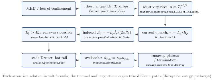
vaft.diagram.disruption_causal_chain()The thermal-quench -> current-quench -> runaway chain as cause and effect.
vaft.diagram.disruption_causal_chain(*, labels=True)Show source vaft/diagram/_disruption.py, lines 231–271
def disruption_causal_chain(*, labels: bool = True) -> Diagram:
    r"""The thermal-quench -> current-quench -> runaway chain as cause and effect.

    Each box a physical state, each arrow the relation that links it to the
    next, named by its ``vaft.formula`` function: loss of confinement ->
    $T_e$ drops (``thermal_quench_temperature``) -> $\eta \propto T_e^{-3/2}$
    rises (``spitzer_resistivity_from_T_e_Z_eff_ln_Lambda``) -> $R_p$ rises
    and $I_p$ decays by L/R (``lr_time_from_L_R``) -> $E_\parallel$ induced
    (``inductive_parallel_electric_field``) -> $E > E_c$
    (``connor_hastie_critical_field``) -> seed (``dreicer_generation_rate``,
    hot tail) -> avalanche (``avalanche_growth_rate``) -> runaway current.
    """
    labels = _check_labels(labels)
    steps = [
        ("MHD / loss of confinement", "", "start"),
        ("thermal quench: $T_e$ drops", "thermal\\_quench\\_temperature", "tq"),
        ("resistivity rises, $\\eta \\propto T_e^{-3/2}$", "spitzer\\_resistivity\\_from\\_T\\_e\\_Z\\_eff\\_ln\\_Lambda",
         "eta"),
        ("current quench, $\\tau = L_p/R_p$", "lr\\_time\\_from\\_L\\_R", "cq"),
        ("induced $E_\\parallel = -L_p\\dot I_p/(2\\pi R_0)$", "inductive\\_parallel\\_electric\\_field", "E"),
        ("$E_\\parallel > E_c$: runaways possible", "connor\\_hastie\\_critical\\_field", "Ec"),
        ("seed: Dreicer, hot tail", "dreicer\\_generation\\_rate", "seed"),
        ("avalanche: $\\dot n_\\mathrm{RE} = \\gamma_\\mathrm{av}n_\\mathrm{RE}$", "avalanche\\_growth\\_rate", "aval"),
        ("runaway plateau / termination", "runaway\\_current\\_from\\_density", "plateau"),
    ]
    items: List = []
    boxes = []
    for i, (text, fn, role) in enumerate(steps):
        col, row = i % 3, i // 3
        x = 2.6 + 5.4 * col if row % 2 == 0 else 2.6 + 5.4 * (2 - col)
        y = -2.4 * row
        b = box(x, y, 5.0, 1.3, text + (f"\\\\ {{\\scriptsize\\texttt{{{fn}}}}}" if (fn and labels) else ""),
                role=f"step:{role}", latex=True)
        boxes.append(b)
        items += list(b.items)
    for a, b in zip(boxes[:-1], boxes[1:]):
        items.append(connector(a, b, role="edge"))
    if labels:
        items.append(_note("Each arrow is a relation in vaft.formula; the thermal and magnetic energies take "
                           "different paths (disruption\\_energy\\_pathways)", 8.0, -6.0))
    return Diagram("disruption_causal_chain", Scene(tuple(items)), model={"steps": [s[2] for s in steps]})
Formats .svg .tex .pdf the SVG above is committed; build the others locally
import vaft.diagram

d = vaft.diagram.disruption_causal_chain()
d.tikz  # the TikZ document as text
d.save("disruption_causal_chain.svg")  # rendered vector image, the canonical artifact; needs latex, dvisvgm
d.save("disruption_causal_chain.tex")  # the complete TikZ document, the text source
d.save("disruption_causal_chain.pdf")  # vector PDF; needs pdflatex
runaway_generation
1 asset
source
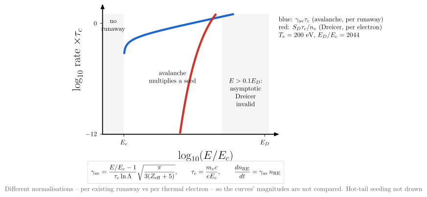
vaft.diagram.runaway_generation()Dreicer and avalanche generation against the field, and the regimes they define.
vaft.diagram.runaway_generation(*, labels=True)Show source vaft/diagram/_disruption.py, lines 274–334
def runaway_generation(*, labels: bool = True) -> Diagram:
    r"""Dreicer and avalanche generation against the field, and the regimes they define.

    For $n_e = 5\times10^{19}$ m$^{-3}$, $T_e = 200$ eV, $Z_\mathrm{eff} = 1.5$:
    $\log_{10}$ of the avalanche growth rate $\gamma_\mathrm{av}\tau_c$
    (``avalanche_growth_rate``, zero below $E_c$) and of the Dreicer rate per
    electron $S_D\tau_c/n_e$ (``dreicer_generation_rate``) against
    $\log_{10}(E/E_c)$. Below $E_c$ nothing runs away; between $E_c$ and a
    few per cent of $E_D$ only an existing seed multiplies; towards $E_D$
    the thermal tail itself runs away. The hot-tail seed of a fast quench is
    not drawn.
    """
    labels = _check_labels(labels)
    n_e, T_e, Z, lnr, lnt = 5e19, 200.0, 1.5, 15.0, 12.0
    E_c = float(connor_hastie_critical_field(n_e, lnr))
    tau_c = float(relativistic_collision_time(n_e, lnr))
    E_D = float(dreicer_field(n_e, T_e, lnt))
    x = np.linspace(-0.5, math.log10(E_D / E_c) + 0.1, 400)
    E = E_c * 10.0**x
    aval = avalanche_growth_rate(E, E_c, Z, lnr) * tau_c
    dre = dreicer_generation_rate(n_e, T_e, E, Z, lnt, prefactor=1.0) * tau_c / n_e
    valid = E <= 0.1 * E_D  # the asymptotic Dreicer formula's own range
    floor = -12.0
    chart = Chart(x_range=(float(x[0]), float(x[-1])), y_range=(floor, 1.0))
    keep_a = aval > 10.0**floor
    keep_d = (dre > 10.0**floor) & valid
    chart.curves.update({"avalanche": np.stack([x[keep_a], np.log10(aval[keep_a])], -1),
                         "dreicer": np.stack([x[keep_d], np.log10(dre[keep_d])], -1)})
    xd = math.log10(E_D / E_c)
    scene = render_chart(chart, x_label="$\\log_{10}(E/E_c)$", y_label="$\\log_{10}$ rate $\\times\\tau_c$",
                         curve_styles={"avalanche": "component imag", "dreicer": "component real"}, region_text={},
                         x_ticks=(0.0, xd), x_tick_text=("$E_c$", "$E_D$"), y_ticks=(floor, 0.0),
                         y_tick_text=(f"${floor:g}$", "$0$"))
    items: List = []
    x_c = float(chart.to_cm(np.array([0.0, 0.0]))[0])
    x_v = float(chart.to_cm(np.array([math.log10(0.1 * E_D / E_c), 0.0]))[0])
    items.append(Polyline.of([(0.0, 0.0), (x_c, 0.0), (x_c, CHART_HEIGHT), (0.0, CHART_HEIGHT)], "concept band",
                             role="regime:none", closed=True))
    items.append(Polyline.of([(x_v, 0.0), (CHART_WIDTH, 0.0), (CHART_WIDTH, CHART_HEIGHT), (x_v, CHART_HEIGHT)],
                             "concept band", role="regime:dreicer_invalid", closed=True))
    items += list(scene.items)
    if labels:
        items += [
            Label((0.5 * x_c, CHART_HEIGHT - 0.2), "no\\\\ runaway", "small label,align=center", anchor="north",
                  role="regime:none"),
            Label((0.42 * CHART_WIDTH, 0.55 * CHART_HEIGHT), "avalanche\\\\ multiplies a seed", "small label,align=center",
                  anchor="north", role="regime:avalanche"),
            Label((0.5 * (x_v + CHART_WIDTH), 0.35 * CHART_HEIGHT), "$E > 0.1E_D$:\\\\ asymptotic\\\\ Dreicer\\\\ "
                  "invalid", "small label,align=center", anchor="center", role="regime:dreicer_invalid"),
            Label((CHART_WIDTH + 0.4, CHART_HEIGHT), "blue: $\\gamma_\\mathrm{av}\\tau_c$ (avalanche, per runaway)"
                  "\\\\ red: $S_D\\tau_c/n_e$ (Dreicer, per electron)\\\\ "
                  f"$T_e = {T_e:g}$ eV, $E_D/E_c = {E_D / E_c:.0f}$", "small label,align=left",
                  anchor="north west", role="legend"),
            Label((CHART_WIDTH / 2, -1.45), f"$\\displaystyle {formula_equation(avalanche_growth_rate)}$",
                  "formula box", anchor="north", role="equations"),
            _note("Different normalisations -- per existing runaway vs per thermal electron -- so the curves' "
                  "magnitudes are not compared. Hot-tail seeding not drawn", CHART_WIDTH / 2 + 1.5, -2.7),
        ]
    return Diagram("runaway_generation", Scene(tuple(items)),
                   model={"E_c": E_c, "E_D": E_D, "tau_c": tau_c, "x": x, "avalanche": aval, "dreicer": dre,
                          "dreicer_drawn": x[keep_d]})
Formats .svg .tex .pdf the SVG above is committed; build the others locally
import vaft.diagram

d = vaft.diagram.runaway_generation()
d.tikz  # the TikZ document as text
d.save("runaway_generation.svg")  # rendered vector image, the canonical artifact; needs latex, dvisvgm
d.save("runaway_generation.tex")  # the complete TikZ document, the text source
d.save("runaway_generation.pdf")  # vector PDF; needs pdflatex
Formula functions referenced:
disruption.avalanche_growth_rate, disruption.connor_hastie_critical_field, disruption.dreicer_field, disruption.dreicer_generation_rate, disruption.relativistic_collision_time
disruption_energy_pathways
1 asset
source
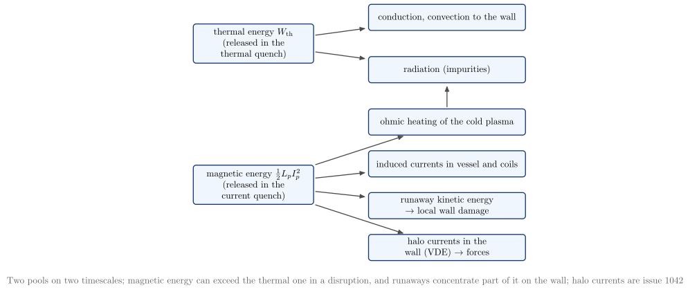
vaft.diagram.disruption_energy_pathways()Where a disruption’s thermal and magnetic energies go.
vaft.diagram.disruption_energy_pathways(*, labels=True)Show source vaft/diagram/_disruption.py, lines 337–377
def disruption_energy_pathways(*, labels: bool = True) -> Diagram:
    r"""Where a disruption's thermal and magnetic energies go.

    The thermal energy $W_\mathrm{th} = \tfrac32\int(n_eT_e + n_iT_i)\,dV$
    leaves in the thermal quench, by conduction and convection to the wall
    and by radiation. The magnetic energy $\tfrac12L_pI_p^2$ of the poloidal
    field leaves in the current quench: ohmically heating the cold plasma
    (and so radiated), inductively coupled into the vessel and coils, and --
    if runaways form -- into their kinetic energy, deposited locally on the
    wall. Two pools, two timescales, different damage mechanisms.
    """
    labels = _check_labels(labels)
    items: List = []
    w_th = box(2.5, 0.0, 4.6, 1.5, "thermal energy $W_\\mathrm{th}$\\\\ (released in the thermal quench)", role="pool:thermal",
               latex=True)
    w_mag = box(2.5, -5.4, 4.6, 1.5, "magnetic energy $\\tfrac12L_pI_p^2$\\\\ (released in the current quench)",
                role="pool:magnetic", latex=True)
    sinks = {
        "conduction": box(9.9, 1.0, 6.0, 1.0, "conduction, convection to the wall", role="sink:conduction",
                          latex=True),
        "radiation": box(9.9, -1.0, 6.0, 1.0, "radiation (impurities)", role="sink:radiation", latex=True),
        "ohmic": box(9.9, -3.0, 6.0, 1.0, "ohmic heating of the cold plasma", role="sink:ohmic", latex=True),
        "vessel": box(9.9, -4.6, 6.0, 1.0, "induced currents in vessel and coils", role="sink:vessel", latex=True),
        "runaway": box(9.9, -6.2, 6.0, 1.0, "runaway kinetic energy $\\to$ local wall damage", role="sink:runaway",
                       latex=True),
        "halo": box(9.9, -7.8, 6.0, 1.0, "halo currents in the wall (VDE) $\\to$ forces", role="sink:halo",
                    latex=True),
    }
    for b in (w_th, w_mag, *sinks.values()):
        items += list(b.items)
    edges = [(w_th, sinks["conduction"]), (w_th, sinks["radiation"]), (w_mag, sinks["ohmic"]),
             (w_mag, sinks["vessel"]), (w_mag, sinks["runaway"]), (w_mag, sinks["halo"]),
             (sinks["ohmic"], sinks["radiation"])]
    for a, b in edges:
        items.append(connector(a, b, role="edge"))
    if labels:
        items.append(_note("Two pools on two timescales; magnetic energy can exceed the thermal one in a "
                           "disruption, and runaways concentrate part of it on the wall; halo currents are issue 1042",
                           6.0, -8.8))
    return Diagram("disruption_energy_pathways", Scene(tuple(items)),
                   model={"pools": ("thermal", "magnetic"), "sinks": tuple(sinks)})
Formats .svg .tex .pdf the SVG above is committed; build the others locally
import vaft.diagram

d = vaft.diagram.disruption_energy_pathways()
d.tikz  # the TikZ document as text
d.save("disruption_energy_pathways.svg")  # rendered vector image, the canonical artifact; needs latex, dvisvgm
d.save("disruption_energy_pathways.tex")  # the complete TikZ document, the text source
d.save("disruption_energy_pathways.pdf")  # vector PDF; needs pdflatex
A prescribed ideal displacement on an arbitrary equilibrium
Module vaft.diagram._mhd_mode
kink_mode
2 assets
source
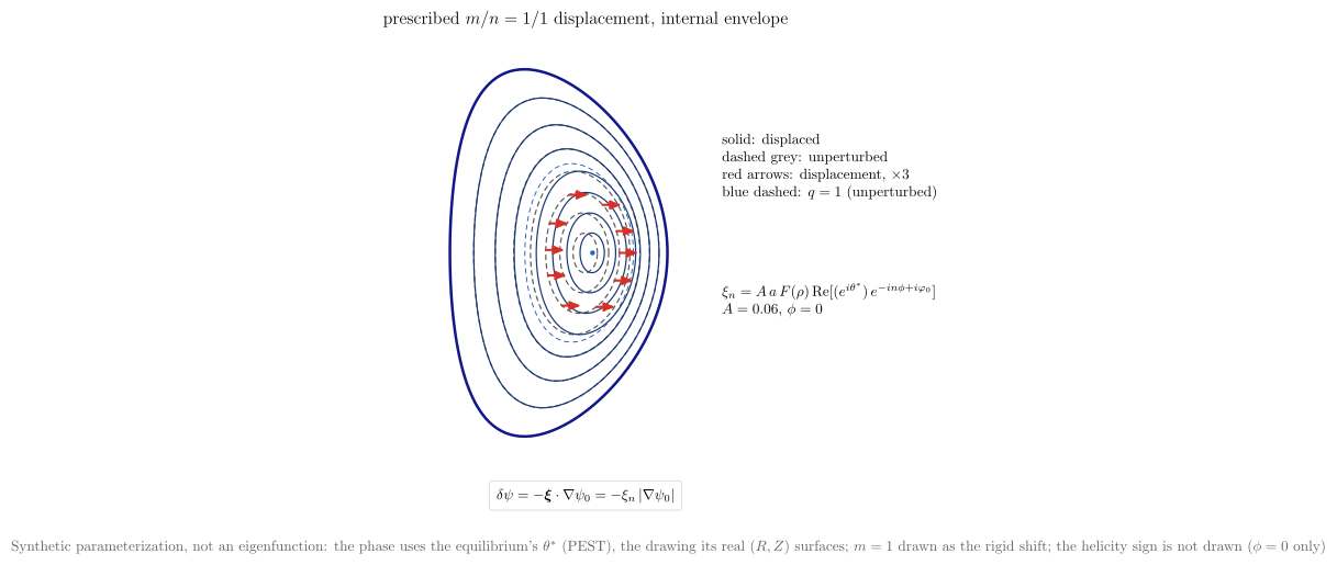
vaft.diagram.kink_mode()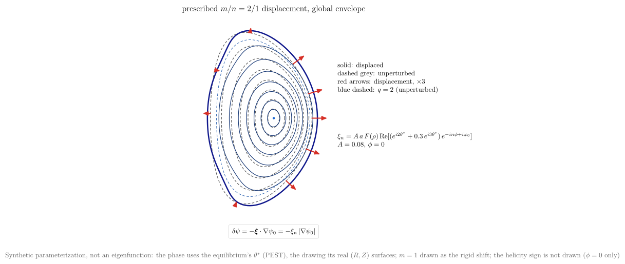
vaft.diagram.kink_mode(m=2, n=1, radial_profile='global', amplitude=0.08, harmonics={2: 1.0, 3: 0.3})A prescribed $m/n$ ideal displacement drawn on an equilibrium’s own flux surfaces.
vaft.diagram.kink_mode(equilibrium=None, m=1, n=1, *, amplitude=0.06, radial_profile='internal', phase=0.0, harmonics=None, labels=True)Formats .svg .tex .pdf the SVG above is committed; build the others locally
import vaft.diagram

d = vaft.diagram.kink_mode()
d.tikz  # the TikZ document as text
d.save("kink_mode_1_1_internal.svg")  # rendered vector image, the canonical artifact; needs latex, dvisvgm
d.save("kink_mode_1_1_internal.tex")  # the complete TikZ document, the text source
d.save("kink_mode_1_1_internal.pdf")  # vector PDF; needs pdflatex
Formula functions referenced:
equilibrium.flux_perturbation_from_normal_displacement
A Kadomtsev-like sawtooth on an arbitrary equilibrium, as three distinct states
Module vaft.diagram._sawtooth
sawtooth
3 assets
source
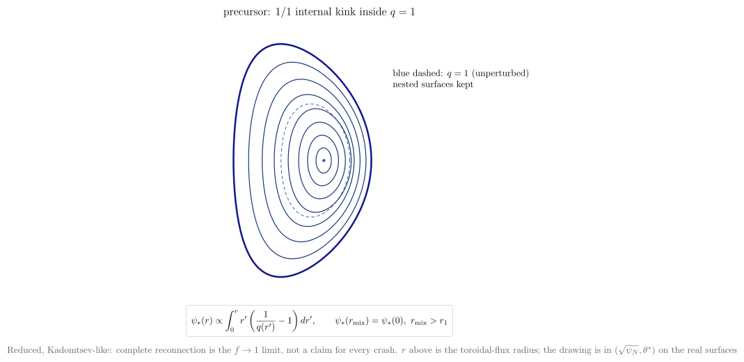
vaft.diagram.sawtooth(stage='precursor')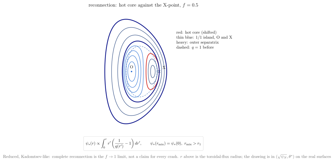
vaft.diagram.sawtooth(stage='reconnection')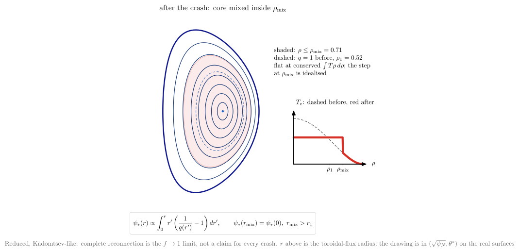
vaft.diagram.sawtooth(stage='post_crash')A reduced, Kadomtsev-like sawtooth crash in one of three states, on an equilibrium’s surfaces.
vaft.diagram.sawtooth(equilibrium=None, stage='precursor', *, amplitude=0.06, reconnection_fraction=0.5, labels=True)Formats .svg .tex .pdf the SVG above is committed; build the others locally
import vaft.diagram

d = vaft.diagram.sawtooth(stage='precursor')
d.tikz  # the TikZ document as text
d.save("sawtooth_precursor.svg")  # rendered vector image, the canonical artifact; needs latex, dvisvgm
d.save("sawtooth_precursor.tex")  # the complete TikZ document, the text source
d.save("sawtooth_precursor.pdf")  # vector PDF; needs pdflatex
Formula functions referenced:
stability.kadomtsev_mixing_radius
Reduced Hamiltonian field-line topology on an arbitrary equilibrium
Module vaft.diagram._magnetic_topology
stochastic_layer
3 assets
source
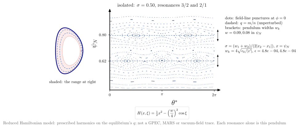
vaft.diagram.stochastic_layer(regime='isolated')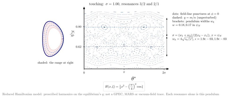
vaft.diagram.stochastic_layer(regime='touching')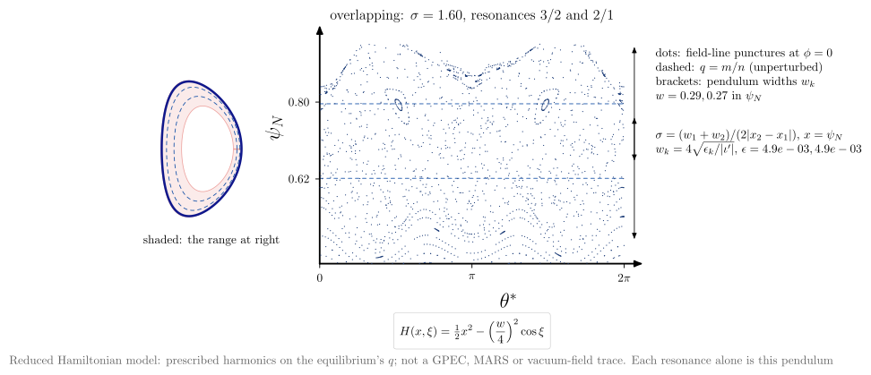
vaft.diagram.stochastic_layer(regime='overlapping')Island overlap on an equilibrium: a Poincare section of two resonant harmonics.
vaft.diagram.stochastic_layer(equilibrium=None, regime='touching', *, resonances=((3, 2), (2, 1)), overlap=None, perturbations=None, labels=True)Formats .svg .tex .pdf the SVG above is committed; build the others locally
import vaft.diagram

d = vaft.diagram.stochastic_layer(regime='isolated')
d.tikz  # the TikZ document as text
d.save("stochastic_layer_isolated.svg")  # rendered vector image, the canonical artifact; needs latex, dvisvgm
d.save("stochastic_layer_isolated.tex")  # the complete TikZ document, the text source
d.save("stochastic_layer_isolated.pdf")  # vector PDF; needs pdflatex
Formula functions referenced:
stability.island_pendulum_hamiltonian
separatrix_lobes
1 asset
source
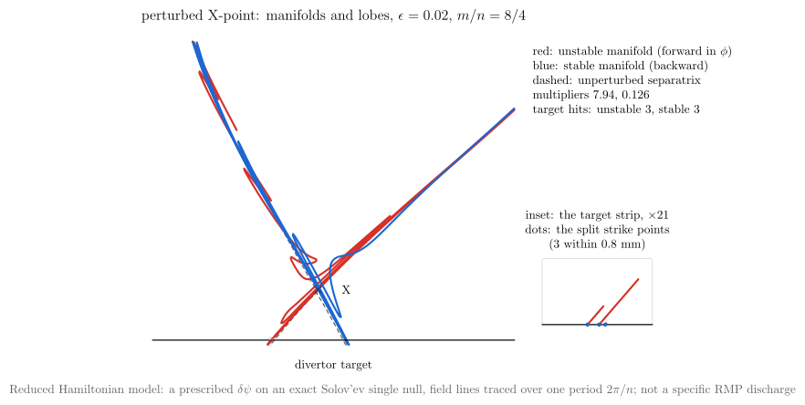
vaft.diagram.separatrix_lobes()Stable and unstable manifolds of a perturbed X-point, and the lobes between them.
vaft.diagram.separatrix_lobes(equilibrium=None, *, perturbation=0.02, m=8, n=4, phase=0.0, labels=True)Formats .svg .tex .pdf the SVG above is committed; build the others locally
import vaft.diagram

d = vaft.diagram.separatrix_lobes()
d.tikz  # the TikZ document as text
d.save("separatrix_lobes.svg")  # rendered vector image, the canonical artifact; needs latex, dvisvgm
d.save("separatrix_lobes.tex")  # the complete TikZ document, the text source
d.save("separatrix_lobes.pdf")  # vector PDF; needs pdflatex
Vertical displacement events: hot and cold VDE, halo currents and timescales
Module vaft.diagram._vde
hot_vde_sequence
1 asset
source
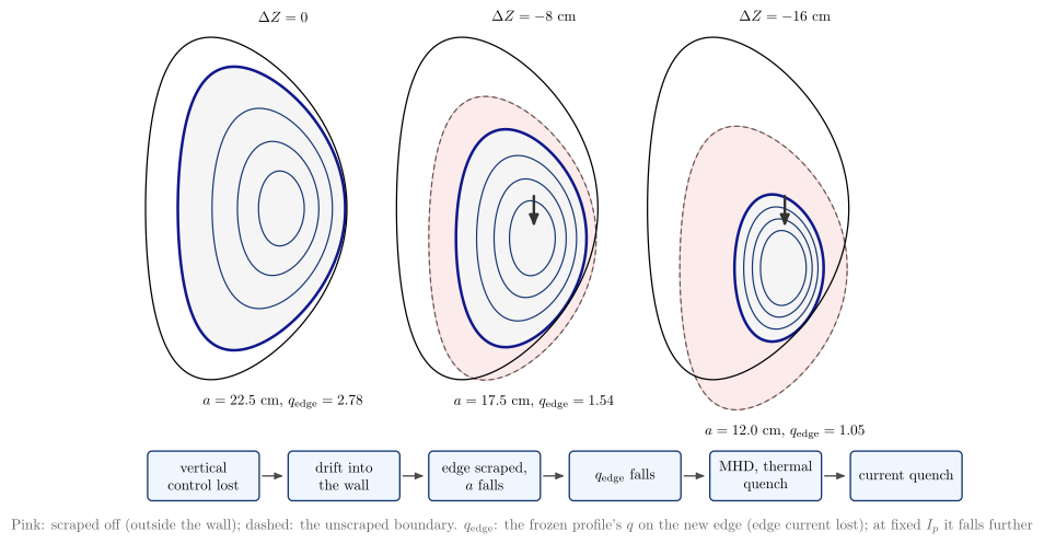
vaft.diagram.hot_vde_sequence()A hot VDE: the plasma drifts into the wall, is scraped, and its edge $q$ falls at constant $I_p$.
vaft.diagram.hot_vde_sequence(*, labels=True)Show source vaft/diagram/_vde.py, lines 106–166
def hot_vde_sequence(*, labels: bool = True) -> Diagram:
    r"""A hot VDE: the plasma drifts into the wall, is scraped, and its edge $q$ falls at constant $I_p$.

    Three frames of the default Solov'ev plasma moved down by 0, 8 and 16 cm
    inside its limiter (``hot_vde_frames``): the limiting surface is the
    largest flux surface that still fits, the scraped part shaded. The edge
    moves inward to a surface of lower $q$ (the frozen profile's; at fixed
    $I_p$, the hot-VDE assumption before the quench, lower still),
    towards the MHD limit. The displacement
    can trigger the thermal quench, not the other way round. Below, the
    causal chain.
    """
    labels = _check_labels(labels)
    data = hot_vde_frames()
    geom = data["geometry"]
    eq = geom.equilibrium
    wall = np.stack([np.asarray(eq.limiter.r, float), np.asarray(eq.limiter.z, float)], -1)
    lcfs = geom.surface(0.97)
    items: List = []
    width = _S * (float(wall[:, 0].max() - wall[:, 0].min())) + 1.2
    for i, f in enumerate(data["frames"]):
        ox = i * width - _S * float(wall[:, 0].min())

        def cm(R, Z, ox=ox):
            return np.stack([ox + _S * np.asarray(R), _S * np.asarray(Z)], -1)

        items.append(Polyline.of(cm(lcfs.R, lcfs.Z - f["shift"]), "layer", role="scraped", closed=True))
        s = geom.surface(f["rho"])
        items.append(Polyline.of(cm(s.R, s.Z - f["shift"]), "concept band", role="kept", closed=True))
        items.append(Polyline.of(cm(lcfs.R, lcfs.Z - f["shift"]), "approx", role="original_boundary", closed=True))
        for rho in np.linspace(0.3, f["rho"], 4)[:-1]:
            si = geom.surface(float(round(rho, 4)))
            items.append(Polyline.of(cm(si.R, si.Z - f["shift"]), "orbit electron", role="surface", closed=True))
        items.append(Polyline.of(cm(s.R, s.Z - f["shift"]), "boundary", role="limiting_surface", closed=True))
        items.append(Polyline.of(cm(wall[:, 0], wall[:, 1]), "machine", role="wall", closed=True))
        if i:
            c = cm(geom.axis[0], geom.axis[1])
            items.append(Arrow((float(c[0]), float(c[1]) + 0.3), (float(c[0]), float(c[1]) - 0.5), "exb",
                               role="motion"))
        if labels:
            top = _S * float(wall[:, 1].max()) + 0.25
            x_mid = ox + _S * geom.axis[0]
            items.append(Label((x_mid, top), f"$\\Delta Z = {-100 * f['shift']:.0f}$ cm" if f["shift"] else
                               "$\\Delta Z = 0$", "small label", anchor="south", role="title"))
            items.append(Label((x_mid, _S * min(float(wall[:, 1].min()), float(lcfs.Z.min()) - f["shift"]) - 0.25),
                               f"$a = {100 * f['a']:.1f}$ cm, $q_\\mathrm{{edge}} = {f['q_edge']:.2f}$", "small label",
                               anchor="north", role="q_edge"))
    if labels:
        y0 = _S * (float(lcfs.Z.min()) - SHIFTS[-1]) - 1.6
        chain = ["vertical control lost", "drift into the wall", "edge scraped, $a$ falls",
                 "$q_\\mathrm{edge}$ falls", "MHD, thermal quench", "current quench"]
        boxes = [box(1.4 + 3.4 * k, y0, 2.7, 1.2, text, role=f"chain:{k}", latex=True) for k, text in enumerate(chain)]
        for b in boxes:
            items += list(b.items)
        for a_, b_ in zip(boxes[:-1], boxes[1:]):
            items.append(connector(a_, b_, role="chain_edge"))
        items.append(_note("Pink: scraped off (outside the wall); dashed: the unscraped boundary. $q_\\mathrm{edge}$: the "
                           "frozen profile's $q$ on the new edge (edge current lost); at fixed $I_p$ it falls further",
                           1.5 * width, y0 - 0.9))
    # a copy: hot_vde_frames is lru_cached, and a caller's edit must not reach the next build
    return Diagram("hot_vde_sequence", Scene(tuple(items)), model={"frames": copy.deepcopy(data["frames"])})
Formats .svg .tex .pdf the SVG above is committed; build the others locally
import vaft.diagram

d = vaft.diagram.hot_vde_sequence()
d.tikz  # the TikZ document as text
d.save("hot_vde_sequence.svg")  # rendered vector image, the canonical artifact; needs latex, dvisvgm
d.save("hot_vde_sequence.tex")  # the complete TikZ document, the text source
d.save("hot_vde_sequence.pdf")  # vector PDF; needs pdflatex
Formula functions referenced:
geometry.cylindrical_poloidal_field, geometry.cylindrical_safety_factor_from_r_B
cold_vde_bifurcation
1 asset
source
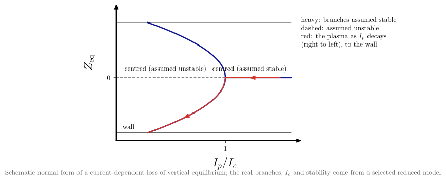
vaft.diagram.cold_vde_bifurcation()Cold VDE as the loss of a centred vertical equilibrium while the current decays (schematic).
vaft.diagram.cold_vde_bifurcation(*, labels=True)Show source vaft/diagram/_vde.py, lines 176–230
def cold_vde_bifurcation(*, labels: bool = True) -> Diagram:
    r"""Cold VDE as the loss of a centred vertical equilibrium while the current decays (schematic).

    After the thermal quench the current decays; below a critical current
    $I_c$ the centred ($Z = 0$) equilibrium stops being stable and two
    off-centre branches $Z = \pm Z_s\sqrt{(I_c - I)/I_c}$ appear
    (``cold_vde_branches``). The plasma, following the decaying current from
    right to left, leaves along one of them into the wall. This is the
    normal form of a symmetric pitchfork drawn to explain the concept; the
    branch structure, $I_c$ and the stability of each branch are properties
    of a selected reduced model (e.g. a current filament with a conducting
    wall), which is not chosen here.
    """
    labels = _check_labels(labels)
    I = np.linspace(0.0, 1.6, 321)
    off = cold_vde_branches(I, 1.0, 1.3)
    chart = Chart(x_range=(0.0, 1.6), y_range=(-1.25, 1.25))
    below = I <= 1.0
    chart.curves.update({
        "centred_stable": np.stack([I[~below], np.zeros((~below).sum())], -1),
        "centred_unstable": np.stack([I[below], np.zeros(below.sum())], -1),
        # the branches end at the walls, |Z| = 1.1
        "upper": np.stack([I[below & (off <= 1.1)], off[below & (off <= 1.1)]], -1),
        "lower": np.stack([I[below & (off <= 1.1)], -off[below & (off <= 1.1)]], -1),
        "wall": np.array([[0.0, -1.1], [1.6, -1.1]]),
        "wall_upper": np.array([[0.0, 1.1], [1.6, 1.1]]),
    })
    scene = render_chart(chart, x_label="$I_p/I_c$", y_label="$Z_\\mathrm{eq}$",
                         curve_styles={"centred_stable": "boundary", "centred_unstable": "approx",
                                       "upper": "boundary", "lower": "boundary", "wall": "machine",
                                       "wall_upper": "machine"},
                         region_text={}, x_ticks=(1.0,), x_tick_text=("$1$",), y_ticks=(0.0,), y_tick_text=("$0$",))
    items: List = list(scene.items)
    # the path the plasma follows as the current decays
    path_I = np.concatenate([np.linspace(1.5, 1.0, 20), np.linspace(1.0, 0.0, 60)])
    path_Z = np.concatenate([np.zeros(20), -cold_vde_branches(np.linspace(1.0, 0.0, 60), 1.0, 1.3)])
    keep = path_Z >= -1.1  # the plasma stops at the wall
    path = chart.to_cm(np.stack([path_I[keep], path_Z[keep]], -1))
    items.append(Polyline.of(path, "trough", role="trajectory"))
    for k in (8, min(40, len(path) - 4)):
        items.append(Arrow(tuple(path[k]), tuple(path[k + 3]), "drift", role="trajectory_direction"))
    if labels:
        wall_y = float(chart.to_cm(np.array([0.0, -1.1]))[1])
        items += [
            Label((CHART_WIDTH - 0.1, float(chart.to_cm(np.array([0.0, 0.0]))[1]) + 0.15), "centred (assumed stable)",
                  "small label", anchor="south east", role="branch"),
            Label((0.3, float(chart.to_cm(np.array([0.0, 0.0]))[1]) + 0.15), "centred (assumed unstable)",
                  "small label", anchor="south west", role="branch"),
            Label((0.2, wall_y + 0.08), "wall", "small label", anchor="south west", role="wall"),
            Label((CHART_WIDTH + 0.4, CHART_HEIGHT), "heavy: branches assumed stable\\\\ dashed: assumed unstable\\\\ red: the plasma "
                  "as $I_p$ decays\\\\ (right to left), to the wall", "small label,align=left", anchor="north west", role="legend"),
            _note("Schematic normal form of a current-dependent loss of vertical equilibrium; the real branches, "
                  "$I_c$ and stability come from a selected reduced model", CHART_WIDTH / 2 + 1.0, -1.4),
        ]
    return Diagram("cold_vde_bifurcation", Scene(tuple(items)), model={"I": I, "off": off, "I_crit": 1.0})
Formats .svg .tex .pdf the SVG above is committed; build the others locally
import vaft.diagram

d = vaft.diagram.cold_vde_bifurcation()
d.tikz  # the TikZ document as text
d.save("cold_vde_bifurcation.svg")  # rendered vector image, the canonical artifact; needs latex, dvisvgm
d.save("cold_vde_bifurcation.tex")  # the complete TikZ document, the text source
d.save("cold_vde_bifurcation.pdf")  # vector PDF; needs pdflatex
plasma_wall_halo_current
1 asset
source
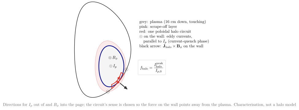
vaft.diagram.plasma_wall_halo_current()Wall contact in a VDE: one halo-current circuit, the eddy currents, and the force on the wall.
vaft.diagram.plasma_wall_halo_current(*, labels=True)Show source vaft/diagram/_vde.py, lines 311–371
def plasma_wall_halo_current(*, labels: bool = True) -> Diagram:
    r"""Wall contact in a VDE: one halo-current circuit, the eddy currents, and the force on the wall.

    The 16 cm hot-VDE frame, its limiting surface touching the lower
    outboard limiter. One poloidal halo circuit (``halo_circuit``) leaves the
    plasma edge into the scrape-off layer, runs through the wall and returns;
    its sense is set so that $\mathbf J_\mathrm{halo}\times\mathbf B_\phi$ on
    the wall segment -- with $B_\phi$ into the page, $\otimes$ -- points out of
    the plasma, the measured sense of the halo load. $I_p$ is drawn out of the
    page ($\odot$); in the current-quench phase shown, the wall's eddy
    currents run parallel to it ($\odot$). Not a halo-current model:
    ``halo_current_fraction`` and ``toroidal_peaking_factor`` characterise one.
    """
    labels = _check_labels(labels)
    h = halo_circuit()
    geom = hot_vde_frames()["geometry"]
    frame = h["frame"]
    items: List = []

    def cm(pts):
        return _S * np.asarray(pts, dtype=float)

    halo = geom.surface(min(0.97, frame["rho"] + 0.12))
    items.append(Polyline.of(cm(np.stack([halo.R, halo.Z - frame["shift"]], -1)), "layer", role="halo_region",
                             closed=True))
    items.append(Polyline.of(cm(h["edge"]), "concept band", role="plasma", closed=True))
    items.append(Polyline.of(cm(h["edge"]), "boundary", role="plasma_boundary", closed=True))
    items.append(Polyline.of(cm(h["wall"]), "machine", role="wall", closed=True))
    items.append(Polyline.of(cm(h["circuit"]), "trough", role="halo_current"))
    c = h["circuit"]
    n_wall = 1 + len(h["wall_path"])
    for a, b in ((c[n_wall // 2 - 1], c[n_wall // 2]), (c[n_wall + (len(c) - n_wall) // 2 - 1],
                                                         c[n_wall + (len(c) - n_wall) // 2])):
        mid = 0.5 * (a + b)
        step = 0.35 * (b - a) / max(np.linalg.norm(b - a), 1e-12) / _S
        items.append(Arrow(tuple(cm(mid - step)), tuple(cm(mid + step)), "drift", role="halo_current_direction"))
    mid = c[n_wall // 2]
    items.append(Arrow(tuple(cm(mid) + 0.2 * h["force"]), tuple(cm(mid) + 1.1 * h["force"]), "exb", role="force"))
    axis = np.array(geom.axis) - np.array([0.0, frame["shift"]])
    items.append(Label(tuple(cm(axis)), "$\\odot\\,I_p$", "small label", role="plasma_current"))
    items.append(Label(tuple(cm(axis + np.array([0.0, 0.08]))), "$\\otimes\\,B_\\phi$", "small label",
                       role="toroidal_field"))
    for k in (-3, 3):
        p = h["wall"][(int(np.argmin(np.linalg.norm(h["wall"] - h["contact"], axis=1))) + 12 * k) % len(h["wall"])]
        items.append(Label(tuple(cm(p)), "$\\odot$", "charge small", role="eddy_current"))
    if labels:
        right = _S * float(h["wall"][:, 0].max()) + 0.6
        items += [
            Label((right, _S * 0.3), "grey: plasma (16 cm down, touching)\\\\ pink: scrape-off layer\\\\ "
                  "red: one poloidal halo circuit\\\\ $\\odot$ on the wall: eddy currents,\\\\ \\quad parallel to "
                  "$I_p$ (current-quench phase)\\\\ black arrow: $\\mathbf{J}_\\mathrm{halo}\\times\\mathbf{B}_\\phi$ "
                  "on the wall", "small label,align=left", anchor="north west", role="legend"),
            Label((right, -_S * 0.1), f"$\\displaystyle {formula_equation(halo_current_fraction)}$", "formula box",
                  anchor="north west", role="equations"),
            _note("Directions for $I_p$ out of and $B_\\phi$ into the page; the circuit's sense is chosen so the "
                  "force on the wall points away from the plasma. Characterisation, not a halo model",
                  right + 1.0, -_S * 0.5),
        ]
    return Diagram("plasma_wall_halo_current", Scene(tuple(items)),
                   model={"shift": frame["shift"], "rho": frame["rho"], "circuit": h["circuit"],
                          "force": h["force"], "normal_out": h["normal_out"], "wall_tangent": h["wall_tangent"]})
Formats .svg .tex .pdf the SVG above is committed; build the others locally
import vaft.diagram

d = vaft.diagram.plasma_wall_halo_current()
d.tikz  # the TikZ document as text
d.save("plasma_wall_halo_current.svg")  # rendered vector image, the canonical artifact; needs latex, dvisvgm
d.save("plasma_wall_halo_current.tex")  # the complete TikZ document, the text source
d.save("plasma_wall_halo_current.pdf")  # vector PDF; needs pdflatex
Formula functions referenced:
geometry.cylindrical_poloidal_field, geometry.cylindrical_safety_factor_from_r_B, vde.halo_current_fraction
vde_timescales
1 asset
source
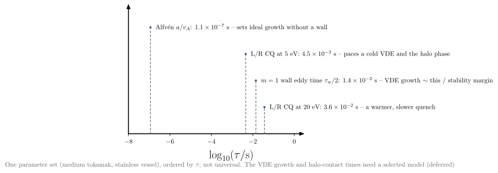
vaft.diagram.vde_timescales()The VDE’s timescales on one log axis, for one parameter set.
vaft.diagram.vde_timescales(*, labels=True)Show source vaft/diagram/_vde.py, lines 394–431
def vde_timescales(*, labels: bool = True) -> Diagram:
    r"""The VDE's timescales on one log axis, for one parameter set.

    The Alfvenic time $a/v_A$ (``v_alfven_from_B_n_mi``) sets ideal vertical
    growth without a wall; the $m = 1$ eddy time of a thin stainless vessel
    (``thin_wall_time``, ``wall_mode_decay_time``) slows it to a wall-mediated
    VDE; the L/R current-quench time at 5 and 20 eV (Spitzer resistivity,
    ``startup`` circuit) paces a cold VDE and the halo phase. One generic
    medium tokamak ($R_0 = 1.7$ m, 2 T, $5\times10^{19}$ m$^{-3}$, 2 cm steel
    at 0.8 m): the ordering is this set's, not universal.
    """
    labels = _check_labels(labels)
    t = vde_timescales_table()
    rows = [("tau_A", "Alfv\\'en $a/v_A$", "sets ideal growth without a wall"),
            ("tau_CQ_5eV", "L/R CQ at 5 eV", "paces a cold VDE and the halo phase"),
            ("tau_wall_m1", "$m = 1$ wall eddy time $\\tau_w/2$", "VDE growth $\\sim$ this / stability margin"),
            ("tau_CQ_20eV", "L/R CQ at 20 eV", "a warmer, slower quench")]
    lo, hi = -8.0, 0.0
    chart = Chart(x_range=(lo, hi), y_range=(0.0, len(rows) + 0.5))
    scene = render_chart(chart, x_label="$\\log_{10}(\\tau/\\mathrm{s})$", y_label="", curve_styles={},
                         region_text={}, x_ticks=tuple(float(v) for v in range(-8, 1, 2)),
                         x_tick_text=tuple(f"${v}$" for v in range(-8, 1, 2)))
    items: List = list(scene.items)
    for k, (key, _name, _regime) in enumerate(rows):
        at = chart.to_cm(np.array([math.log10(t[key]), len(rows) - k]))
        items.append(Marker((float(at[0]), float(at[1])), "o", "opoint", role=f"tau:{key}"))
        items.append(Polyline.of([(float(at[0]), 0.0), (float(at[0]), float(at[1]))], "approx", role=f"tau:{key}"))
    if labels:
        for k, (key, name, regime) in enumerate(rows):
            end = chart.to_cm(np.array([math.log10(t[key]), len(rows) - k]))
            mant, expo = f"{t[key]:.1e}".split("e")
            items.append(Label((float(end[0]) + 0.15, float(end[1])),
                               f"{name}: ${mant}\\times10^{{{int(expo)}}}$ s -- {regime}", "small label",
                               anchor="west", role=f"row:{key}"))
        items.append(_note("One parameter set (medium tokamak, stainless vessel), ordered by $\\tau$; not universal. "
                           "The VDE growth and halo-contact times need a selected model (deferred)", CHART_WIDTH / 2 + 1.0,
                           -1.4))
    return Diagram("vde_timescales", Scene(tuple(items)), model=t)
Formats .svg .tex .pdf the SVG above is committed; build the others locally
import vaft.diagram

d = vaft.diagram.vde_timescales()
d.tikz  # the TikZ document as text
d.save("vde_timescales.svg")  # rendered vector image, the canonical artifact; needs latex, dvisvgm
d.save("vde_timescales.tex")  # the complete TikZ document, the text source
d.save("vde_timescales.pdf")  # vector PDF; needs pdflatex
Formula functions referenced:
equilibrium.spitzer_resistivity_from_T_e_Z_eff_ln_Lambda, stability.v_alfven_from_B_n_mi, startup.lr_time_from_L_R, startup.plasma_inductance_circular_from_R0_a_li, startup.plasma_resistance_uniform_ellipse_from_eta_R0_a_kappa, vde.thin_wall_time, vde.wall_mode_decay_time
The Grad–Shafranov problem: regions, boundaries, topology and problem classes
Module vaft.diagram._gs_equilibrium
grad_shafranov_domain_decomposition
1 asset
source
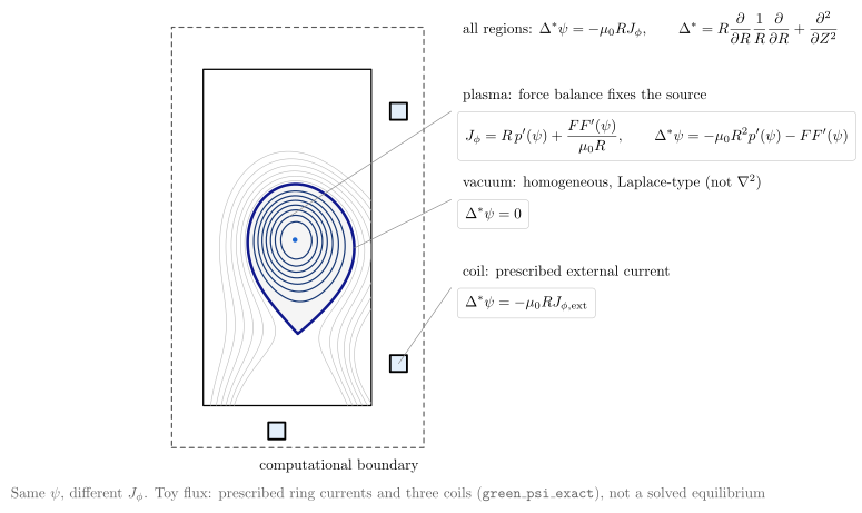
vaft.diagram.grad_shafranov_domain_decomposition()Same flux function, different sources: plasma, vacuum and coil regions of one elliptic problem.
vaft.diagram.grad_shafranov_domain_decomposition(*, labels=True)Show source vaft/diagram/_gs_equilibrium.py, lines 225–273
def grad_shafranov_domain_decomposition(*, labels: bool = True) -> Diagram:
    r"""Same flux function, different sources: plasma, vacuum and coil regions of one elliptic problem.

    The diverted toy equilibrium of ``flux_model``: inside the LCFS (shaded)
    the plasma source of ``toroidal_current_density_from_p_prime_ff_prime``;
    between plasma, coils and the outer boundary the homogeneous equation
    $\Delta^*\psi = 0$; in each coil the prescribed $-\mu_0RJ_{\phi,\mathrm{ext}}$
    -- all ``grad_shafranov_source`` of the region's $J_\phi$. The dashed frame
    is the computational boundary, where a free-boundary code imposes the
    Green's-function flux of all the currents.
    """
    labels = _check_labels(labels)
    model = flux_model("diverted")
    o = (0.0, 0.0)
    boundary = lcfs(model)
    items: List = [Polyline.of(_cm(boundary, o), "concept band", role="region:plasma", closed=True)]
    items += _vessel_items(o, limiter=False)
    items += _surfaces(model, o)
    items.append(Polyline.of(_cm(boundary, o), "boundary", role="lcfs", closed=True))
    items += _coil_items(model["coils"], o)
    r0, r1, z0, z1 = float(_GRID_R[0]), float(_GRID_R[-1]), float(_GRID_Z[0]), float(_GRID_Z[-1])
    items.append(Polyline.of(_cm([(r0, z0), (r1, z0), (r1, z1), (r0, z1)], o), "approx", role="computational_boundary",
                             closed=True))
    items.append(Marker(tuple(_cm(model["axis"], o)), "o", "opoint", role="axis"))
    if labels:
        xr = _S * r1 + 0.8
        rows = [
            ((_R0, 0.1), 3.0, "plasma: force balance fixes the source",
             f"$\\displaystyle {formula_equation(toroidal_current_density_from_p_prime_ff_prime)}$", "plasma"),
            ((0.97, -0.05), 0.9, "vacuum: homogeneous, Laplace-type (not $\\nabla^2$)",
             "$\\displaystyle \\Delta^*\\psi = 0$", "vacuum"),
            (model["coils"][1][:2], -1.2, "coil: prescribed external current",
             "$\\displaystyle \\Delta^*\\psi = -\\mu_0 R J_{\\phi,\\mathrm{ext}}$", "coil"),
        ]
        for point, y, head, eq, role in rows:
            p = _cm(point, o)
            items += [Polyline.of([tuple(p), (xr - 0.15, y)], "leader line", role=f"leader:{role}"),
                      Label((xr, y + 0.1), head, "small label", anchor="south west", role=f"region:{role}"),
                      Label((xr, y), eq, "formula box", anchor="north west", role="equations")]
        items += [
            Label((xr, 5.0), f"all regions: $\\displaystyle {formula_equation(grad_shafranov_source)}$",
                  "small label", anchor="west", role="equations"),
            Label(tuple(_cm((r1, z0), o) + [0.0, -0.15]), "computational boundary", "small label",
                  anchor="north east", role="computational_boundary"),
            _note("Same $\\psi$, different $J_\\phi$. Toy flux: prescribed ring currents and three coils "
                  "(\\texttt{green\\_psi\\_exact}), not a solved equilibrium", 0.5 * (xr + 4.0), _S * z0 - 0.8),
        ]
    return Diagram("grad_shafranov_domain_decomposition", Scene(tuple(items)),
                   model={k: model[k] for k in ("axis", "x_point", "psi_boundary", "limited_by")})
Formats .svg .tex .pdf the SVG above is committed; build the others locally
import vaft.diagram

d = vaft.diagram.grad_shafranov_domain_decomposition()
d.tikz  # the TikZ document as text
d.save("grad_shafranov_domain_decomposition.svg")  # rendered vector image, the canonical artifact; needs latex, dvisvgm
d.save("grad_shafranov_domain_decomposition.tex")  # the complete TikZ document, the text source
d.save("grad_shafranov_domain_decomposition.pdf")  # vector PDF; needs pdflatex
Formula functions referenced:
equilibrium.grad_shafranov_source, equilibrium.toroidal_current_density_from_p_prime_ff_prime, green.green_psi_exact
fixed_vs_free_boundary_equilibrium
1 asset
source
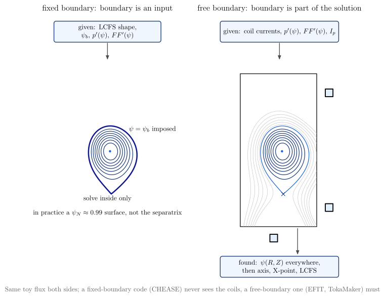
vaft.diagram.fixed_vs_free_boundary_equilibrium()The boundary as an input against the boundary as part of the solution.
vaft.diagram.fixed_vs_free_boundary_equilibrium(*, labels=True)Show source vaft/diagram/_gs_equilibrium.py, lines 276–326
def fixed_vs_free_boundary_equilibrium(*, labels: bool = True) -> Diagram:
    r"""The boundary as an input against the boundary as part of the solution.

    Left, fixed boundary: the LCFS is given (thick) with $\psi = \psi_b$ on
    it, and only the plasma inside is solved -- nothing outside exists for the
    problem. Right, free boundary: coil currents and the plasma source give
    $\psi(R, Z)$ everywhere, and the LCFS -- here through an X-point -- is
    read off the solution's topology. Same toy flux as ``flux_model``.
    """
    labels = _check_labels(labels)
    model = flux_model("diverted")
    boundary = lcfs(model)
    left, right = (0.0, 0.0), (9.0, 0.0)
    items: List = []
    # fixed: the given boundary and the inside only
    items += _surfaces(model, left, inside_only=True)
    items.append(Polyline.of(_cm(boundary, left), "boundary", role="given_boundary", closed=True))
    items.append(Marker(tuple(_cm(model["axis"], left)), "o", "opoint", role="axis"))
    # free: everything, the boundary found
    items += _vessel_items(right, limiter=False)
    items += _surfaces(model, right)
    items += _coil_items(model["coils"], right)
    items.append(Polyline.of(_cm(boundary, right), "separatrix", role="found_boundary", closed=True))
    items.append(Marker(tuple(_cm(model["x_point"], right)), "x", "xpoint", role="x_point"))
    items.append(Marker(tuple(_cm(model["axis"], right)), "o", "opoint", role="axis"))
    if labels:
        top = _S * 0.8 + 1.0
        items.append(Label((_S * _R0, -_S * 0.6), "in practice a $\\psi_N \\approx 0.99$ surface, not the "
                           "separatrix", "small label", anchor="north", role="note:practice"))
        fixed_in = box(_S * _R0, top + 1.2, 5.6, 1.1, "given: LCFS shape, $\\psi_b$, $p'(\\psi)$, $FF'(\\psi)$",
                       role="fixed:input", latex=True)
        free_in = box(right[0] + _S * _R0, top + 1.2, 6.2, 1.1,
                      "given: coil currents, $p'(\\psi)$, $FF'(\\psi)$, $I_p$", role="free:input", latex=True)
        free_out = box(right[0] + _S * _R0, -_S * 0.92 - 1.5, 6.2, 1.1,
                       "found: $\\psi(R, Z)$ everywhere, then axis, X-point, LCFS", role="free:output", latex=True)
        items += list(fixed_in.items) + list(free_in.items) + list(free_out.items)
        items += [Arrow((_S * _R0, top + 0.6), (_S * _R0, top - 0.3), "connector", role="flow"),
                  Arrow((right[0] + _S * _R0, top + 0.6), (right[0] + _S * _R0, top - 0.3), "connector", role="flow"),
                  Arrow((right[0] + _S * 0.85, -_S * 0.8 - 0.1), (right[0] + _S * 0.85, -_S * 0.92 - 0.9),
                        "connector", role="flow"),
                  Label((_S * _R0, top + 2.1), "fixed boundary: boundary is an input", "label", anchor="south",
                        role="title"),
                  Label((right[0] + _S * _R0, top + 2.1), "free boundary: boundary is part of the solution", "label",
                        anchor="south", role="title"),
                  Label(tuple(_cm((_R0 + 0.2, 0.22), left)), "$\\psi = \\psi_b$ imposed", "small label",
                        anchor="west", role="given_boundary"),
                  Label((_S * _R0, -_S * 0.45), "solve inside only", "small label", anchor="north", role="note"),
                  _note("Same toy flux both sides; a fixed-boundary code (CHEASE) never sees the coils, "
                        "a free-boundary one (EFIT, TokaMaker) must", 0.5 * (right[0] + _S * 1.3), -_S * 0.92 - 2.4)]
    return Diagram("fixed_vs_free_boundary_equilibrium", Scene(tuple(items)),
                   model={"boundary": boundary, "x_point": model["x_point"], "axis": model["axis"]})
Formats .svg .tex .pdf the SVG above is committed; build the others locally
import vaft.diagram

d = vaft.diagram.fixed_vs_free_boundary_equilibrium()
d.tikz  # the TikZ document as text
d.save("fixed_vs_free_boundary_equilibrium.svg")  # rendered vector image, the canonical artifact; needs latex, dvisvgm
d.save("fixed_vs_free_boundary_equilibrium.tex")  # the complete TikZ document, the text source
d.save("fixed_vs_free_boundary_equilibrium.pdf")  # vector PDF; needs pdflatex
Formula functions referenced:
green.green_psi_exact
limiter_and_diverted_topologies
1 asset
source
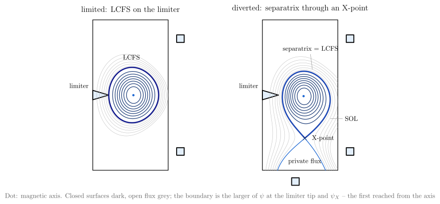
vaft.diagram.limiter_and_diverted_topologies()Where the plasma ends: limiter contact against an X-point separatrix.
vaft.diagram.limiter_and_diverted_topologies(*, labels=True)Show source vaft/diagram/_gs_equilibrium.py, lines 329–387
def limiter_and_diverted_topologies(*, labels: bool = True) -> Diagram:
    r"""Where the plasma ends: limiter contact against an X-point separatrix.

    Two toy equilibria of ``flux_model``, identical but for a divertor coil.
    Limited: the LCFS is the flux surface through the limiter tip, the first
    closed surface to touch a material object. Diverted: the divertor coil
    makes a null of $\nabla\psi$ (X-point) whose flux $\psi_X$ is reached
    before the limiter's, so the separatrix $\psi = \psi_X$ bounds the plasma;
    outside it the scrape-off layer carries open flux to the wall, and below
    the X-point lies the private-flux region.
    """
    labels = _check_labels(labels)
    items: List = []
    info = {}
    for i, configuration in enumerate(CONFIGURATIONS):
        o = (i * 9.0, 0.0)
        model = flux_model(configuration)
        boundary = lcfs(model)
        items += _vessel_items(o)
        items += _surfaces(model, o)
        items.append(Polyline.of(_cm(boundary, o), "boundary", role=f"lcfs:{configuration}", closed=True))
        items.append(Marker(tuple(_cm(model["axis"], o)), "o", "opoint", role="axis"))
        items += _coil_items(model["coils"], o)
        if configuration == "diverted":
            # a hair outside the saddle value: exactly at it the contour joins at the X-point are decided
            # by last-bit differences, which differ between platforms
            level = model["psi_x"] - 1e-6 * (model["psi_axis"] - model["psi_x"])
            for line in _lines(model["psi"], level):
                for run in _clip(line, _VESSEL):
                    items.append(Polyline.of(_cm(run, o), "separatrix", role="separatrix"))
            items.append(Marker(tuple(_cm(model["x_point"], o)), "x", "xpoint", role="x_point"))
        info[configuration] = {"axis": model["axis"], "x_point": model["x_point"], "limited_by": model["limited_by"],
                               "psi_boundary": model["psi_boundary"], "psi_limiter": model["psi_limiter"],
                               "lcfs": boundary}
        if labels:
            title = {"limited": "limited: LCFS on the limiter",
                     "diverted": "diverted: separatrix through an X-point"}[configuration]
            items.append(Label((o[0] + _S * 0.65, _S * 0.8 + 0.3), title, "label", anchor="south", role="title"))
            items += [Label(tuple(_cm((_VESSEL[0], 0.1), o) + [-0.1, 0.0]), "limiter", "small label", anchor="east",
                            role="limiter")]
            if configuration == "limited":
                items.append(Label(tuple(_cm((_R0, _KAPPA * _A + 0.12), o)), "LCFS", "small label", anchor="south",
                                   role="lcfs"))
            else:
                xp = _cm(model["x_point"], o)
                items += [Label(tuple(xp + [0.25, 0.0]), "X-point", "small label", anchor="west", role="x_point"),
                          Label(tuple(xp + [0.0, -0.95]), "private flux", "small label", anchor="north",
                                role="private_flux"),
                          Polyline.of(_cm([(0.97, -0.25), (1.1, -0.25)], o), "leader line", role="sol"),
                          Label(tuple(_cm((1.1, -0.25), o)), "SOL", "small label", anchor="west", role="sol"),
                          Polyline.of(_cm([(_R0 + 0.1, _KAPPA * _A + 0.2), (_R0 + 0.12, _KAPPA * _A + 0.04)], o),
                                      "leader line", role="separatrix"),
                          Label(tuple(_cm((_R0 + 0.1, _KAPPA * _A + 0.2), o)), "separatrix = LCFS", "small label",
                                anchor="south", role="separatrix")]
    if labels:
        items.append(_note("Dot: magnetic axis. Closed surfaces dark, open flux grey; the boundary is the larger of "
                           "$\\psi$ at the limiter tip and $\\psi_X$ -- the first reached from the axis", 8.0,
                           -_S * 0.92 - 0.5))
    return Diagram("limiter_and_diverted_topologies", Scene(tuple(items)), model=info)
Formats .svg .tex .pdf the SVG above is committed; build the others locally
import vaft.diagram

d = vaft.diagram.limiter_and_diverted_topologies()
d.tikz  # the TikZ document as text
d.save("limiter_and_diverted_topologies.svg")  # rendered vector image, the canonical artifact; needs latex, dvisvgm
d.save("limiter_and_diverted_topologies.tex")  # the complete TikZ document, the text source
d.save("limiter_and_diverted_topologies.pdf")  # vector PDF; needs pdflatex
Formula functions referenced:
green.green_psi_exact
equilibrium_problem_taxonomy
1 asset
source
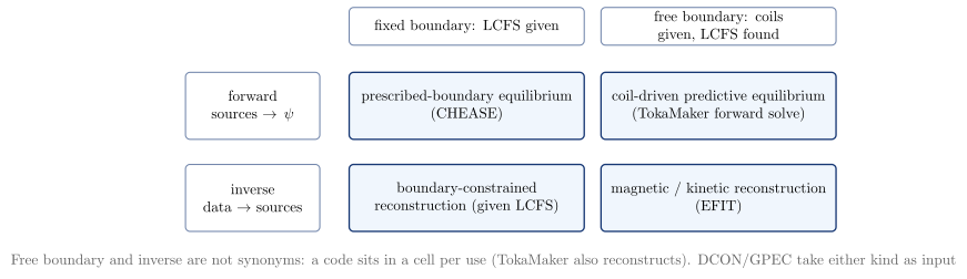
vaft.diagram.equilibrium_problem_taxonomy()Forward/inverse and fixed/free boundary are two axes, not one.
vaft.diagram.equilibrium_problem_taxonomy(*, labels=True)Show source vaft/diagram/_gs_equilibrium.py, lines 390–426
def equilibrium_problem_taxonomy(*, labels: bool = True) -> Diagram:
    r"""Forward/inverse and fixed/free boundary are two axes, not one.

    Rows: forward (profiles and currents given, $\psi$ computed) and inverse
    (measurements given, profiles fitted). Columns: fixed boundary (LCFS
    given) and free boundary (coils given, LCFS found). EFIT is the inverse,
    free-boundary cell; a free-boundary problem need not be inverse
    (TokaMaker's forward solve, as VAFT uses it -- it also has a
    reconstruction mode) and an inverse one need not be free-boundary.
    """
    labels = _check_labels(labels)
    items: List = []
    cells = {
        ("forward", "fixed"): "prescribed-boundary equilibrium\\\\ (CHEASE)",
        ("forward", "free"): "coil-driven predictive equilibrium\\\\ (TokaMaker forward solve)",
        ("inverse", "fixed"): "boundary-constrained\\\\ reconstruction (given LCFS)",
        ("inverse", "free"): "magnetic / kinetic reconstruction\\\\ (EFIT)",
    }
    x_of = {"fixed": 3.2, "free": 9.2}
    y_of = {"forward": 0.0, "inverse": -2.2}
    for (row, col), text in cells.items():
        b = box(x_of[col], y_of[row], 5.6, 1.6, text, role=f"cell:{row}:{col}", latex=True)
        items += list(b.items)
    heads = [box(x_of["fixed"], 1.9, 5.6, 0.9, "fixed boundary: LCFS given", role="axis:fixed", latex=True,
                 style="concept leaf"),
             box(x_of["free"], 1.9, 5.6, 0.9, "free boundary: coils given, LCFS found", role="axis:free", latex=True,
                 style="concept leaf"),
             box(-1.9, y_of["forward"], 3.2, 1.6, "forward\\\\ sources $\\to\\psi$", role="axis:forward", latex=True,
                 style="concept leaf"),
             box(-1.9, y_of["inverse"], 3.2, 1.6, "inverse\\\\ data $\\to$ sources", role="axis:inverse", latex=True,
                 style="concept leaf")]
    for h in heads:
        items += list(h.items)
    if labels:
        items.append(_note("Free boundary and inverse are not synonyms: a code sits in a cell per use (TokaMaker "
                           "also reconstructs). DCON/GPEC take either kind as input", 3.6, y_of["inverse"] - 1.2))
    return Diagram("equilibrium_problem_taxonomy", Scene(tuple(items)), model={"cells": cells})
Formats .svg .tex .pdf the SVG above is committed; build the others locally
import vaft.diagram

d = vaft.diagram.equilibrium_problem_taxonomy()
d.tikz  # the TikZ document as text
d.save("equilibrium_problem_taxonomy.svg")  # rendered vector image, the canonical artifact; needs latex, dvisvgm
d.save("equilibrium_problem_taxonomy.tex")  # the complete TikZ document, the text source
d.save("equilibrium_problem_taxonomy.pdf")  # vector PDF; needs pdflatex
poloidal_flux_source_decomposition
1 asset
source
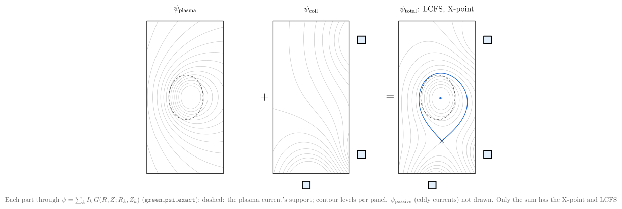
vaft.diagram.poloidal_flux_source_decomposition()$\psi_\mathrm{plasma} + \psi_\mathrm{coil} = \psi_\mathrm{total}$: the topology belongs to the sum.
vaft.diagram.poloidal_flux_source_decomposition(*, labels=True)Show source vaft/diagram/_gs_equilibrium.py, lines 429–476
def poloidal_flux_source_decomposition(*, labels: bool = True) -> Diagram:
    r"""$\psi_\mathrm{plasma} + \psi_\mathrm{coil} = \psi_\mathrm{total}$: the topology belongs to the sum.

    The plasma ring currents and the three coils of the diverted
    ``flux_model``, each through ``green_psi_exact``, and their sum. Neither
    part alone has the X-point or the LCFS; both appear only in the total.
    Passive-structure (eddy) currents would add a further term,
    $\psi_\mathrm{passive}$, not drawn.
    """
    labels = _check_labels(labels)
    model = flux_model("diverted")
    items: List = []
    fields = (("psi_plasma", "plasma"), ("psi_coil", "coil"), ("psi", "total"))
    r0, r1, z0, z1 = _VESSEL
    for i, (key, name) in enumerate(fields):
        o = (i * 6.6, 0.0)
        field = model[key]
        inside = field[np.ix_((_GRID_R >= r0) & (_GRID_R <= r1), (_GRID_Z >= z0) & (_GRID_Z <= z1))]
        lo, hi = np.percentile(inside, [3.0, 97.0])
        for level in np.linspace(lo, hi, 14):
            for line in _lines(field, level):
                for run in _clip(line, _VESSEL):
                    items.append(Polyline.of(_cm(run, o), "surface", role=f"contour:{name}"))
        items.append(Polyline.of(_cm([(r0, z0), (r1, z0), (r1, z1), (r0, z1)], o), "machine", role="vessel",
                                 closed=True))
        if name != "coil":
            items.append(Polyline.of(_cm(np.stack([_R0 + _A * np.cos(np.linspace(0, 2 * math.pi, 61)),
                                                   _KAPPA * _A * np.sin(np.linspace(0, 2 * math.pi, 61))], -1), o),
                                     "approx", role="plasma_current", closed=True))
        if name != "plasma":
            items += _coil_items(model["coils"], o)
        if name == "total":
            items.append(Polyline.of(_cm(lcfs(model), o), "separatrix", role="lcfs", closed=True))
            items.append(Marker(tuple(_cm(model["x_point"], o)), "x", "xpoint", role="x_point"))
            items.append(Marker(tuple(_cm(model["axis"], o)), "o", "opoint", role="axis"))
        if labels:
            text = {"plasma": "$\\psi_\\mathrm{plasma}$", "coil": "$\\psi_\\mathrm{coil}$",
                    "total": "$\\psi_\\mathrm{total}$: LCFS, X-point"}[name]
            items.append(Label((o[0] + _S * 0.65, _S * z1 + 0.3), text, "label", anchor="south", role="title"))
        if i:
            items.append(Label((o[0] + _S * r0 - 0.45, 0.0), "$+$" if i == 1 else "$=$", "legend symbol",
                               role="operator"))
    if labels:
        items.append(_note("Each part through $\\psi = \\sum_k I_k\\,G(R, Z; R_k, Z_k)$ (\\texttt{green\\_psi\\_exact}); "
                           "dashed: the plasma current's support; contour levels per panel. $\\psi_\\mathrm{passive}$ "
                           "(eddy currents) not drawn. Only the sum has the X-point and LCFS", 6.6 + _S * 0.65, -_S * 0.92 - 0.5))
    return Diagram("poloidal_flux_source_decomposition", Scene(tuple(items)),
                   model={"axis": model["axis"], "x_point": model["x_point"]})
Formats .svg .tex .pdf the SVG above is committed; build the others locally
import vaft.diagram

d = vaft.diagram.poloidal_flux_source_decomposition()
d.tikz  # the TikZ document as text
d.save("poloidal_flux_source_decomposition.svg")  # rendered vector image, the canonical artifact; needs latex, dvisvgm
d.save("poloidal_flux_source_decomposition.tex")  # the complete TikZ document, the text source
d.save("poloidal_flux_source_decomposition.pdf")  # vector PDF; needs pdflatex
Formula functions referenced:
green.green_psi_exact
Cylindrical (screw-pinch) geometry: q profile, rational surfaces, mode shapes, matching
Module vaft.diagram._cylindrical_modes
current_to_q_profile
1 asset
source
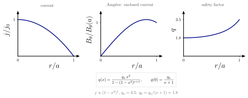
vaft.diagram.current_to_q_profile()From the current profile to the safety factor: $j(r) \to B_\theta(r) \to q(r)$.
vaft.diagram.current_to_q_profile(nu=1.0, q_a=3.5, *, labels=True)Show source vaft/diagram/_cylindrical_modes.py, lines 66–110
def current_to_q_profile(nu: float = _NU, q_a: float = _QA, *, labels: bool = True) -> Diagram:
    r"""From the current profile to the safety factor: $j(r) \to B_\theta(r) \to q(r)$.

    Three panels over $x = r/a$: the current $j \propto (1 - x^2)^\nu$, the
    enclosed-current field $B_\theta \propto [1 - (1 - x^2)^{\nu+1}]/x$ (Ampère),
    and $q(x)$ from ``peaked_current_safety_factor``, which rises from
    $q_a/(\nu + 1)$ on axis: a more peaked current lowers $q_0$ and steepens
    the shear.
    """
    nu, q_a = float(nu), float(q_a)
    if not (0.0 <= nu <= 6.0 and 1.0 <= q_a <= 8.0):
        raise ValueError(f"nu must lie in [0, 6] and q_a in [1, 8], not {nu!r} and {q_a!r}")
    labels = _check_labels(labels)
    x = np.linspace(0.0, 1.0, 201)
    j = (1.0 - x * x) ** nu
    with np.errstate(invalid="ignore", divide="ignore"):
        b = np.where(x > 0, (1.0 - (1.0 - x * x) ** (nu + 1.0)) / np.where(x > 0, x, 1.0), 0.0)
    q = peaked_current_safety_factor(x, q_a, nu)
    panels = [("j", "$j/j_0$", j / j.max()), ("B_theta", "$B_\\theta/B_\\theta(a)$", b / b[-1]),
              ("q", "$q$", q)]
    items: List = []
    charts = {}
    for i, (key, label, y) in enumerate(panels):
        top = 1.15 * float(np.max(y))
        chart = Chart(x_range=(0.0, 1.05), y_range=(0.0, top))
        chart.curves[key] = np.stack([x, y], -1)
        charts[key] = chart
        sub = render_chart(chart, x_label="$r/a$", y_label=label, curve_styles={key: "boundary"}, region_text={},
                           x_ticks=(0.0, 1.0),
                           y_ticks=((1.0,) if key != "q" else ((q_a,) if nu == 0 else (q[0], q_a))),
                           y_tick_text=(("$1$",) if key != "q" else
                                        ((f"${q_a:g}$",) if nu == 0 else (f"${q[0]:.2g}$", f"${q_a:g}$"))))
        items += list(sub.transformed(scale=0.55, offset=(i * 7.0, 0.0)).items)
    if labels:
        for i, text in enumerate(("current", "Ampère: enclosed current", "safety factor")):
            items.append(Label((i * 7.0 + 0.55 * 0.5 * CHART_WIDTH, 0.55 * CHART_HEIGHT + 0.5), text, "subtitle",
                               anchor="south", role="title"))
        items += [
            Label((10.0, -1.4), f"$\\displaystyle {formula_equation(peaked_current_safety_factor)}$", "formula box",
                  anchor="north", role="equations"),
            _note(f"$j \\propto (1 - x^2)^{{{nu:g}}}$, $q_a = {q_a:g}$: $q_0 = q_a/(\\nu + 1) = {q_a / (nu + 1):.2g}$",
                  10.0, -2.8),
        ]
    model = {"nu": nu, "q_a": q_a, "x": x, "j": j, "B_theta": b, "q": q}
    return Diagram("current_to_q_profile", Scene(tuple(items)), model=model)
Formats .svg .tex .pdf the SVG above is committed; build the others locally
import vaft.diagram

d = vaft.diagram.current_to_q_profile()
d.tikz  # the TikZ document as text
d.save("current_to_q_profile.svg")  # rendered vector image, the canonical artifact; needs latex, dvisvgm
d.save("current_to_q_profile.tex")  # the complete TikZ document, the text source
d.save("current_to_q_profile.pdf")  # vector PDF; needs pdflatex
Formula functions referenced:
geometry.peaked_current_safety_factor
cylindrical_rational_surfaces
1 asset
source
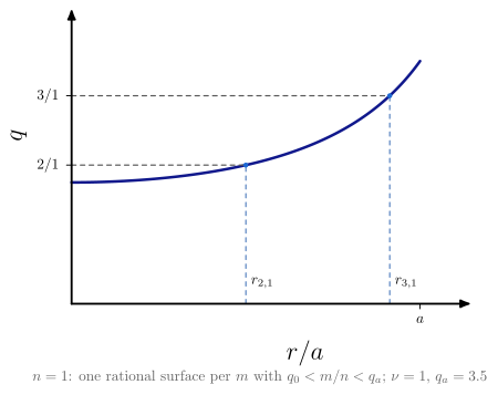
vaft.diagram.cylindrical_rational_surfaces()For one $n$, every $m$ with $q_0 < m/n < q_a$ has its rational surface $q(r_s) = m/n$.
vaft.diagram.cylindrical_rational_surfaces(n=1, *, labels=True)Show source vaft/diagram/_cylindrical_modes.py, lines 113–148
def cylindrical_rational_surfaces(n: int = 1, *, labels: bool = True) -> Diagram:
    r"""For one $n$, every $m$ with $q_0 < m/n < q_a$ has its rational surface $q(r_s) = m/n$.

    $q(r)$ of ``peaked_current_safety_factor`` ($\nu = 1$, $q_a = 3.5$) with
    the levels $m/n$ and their surfaces: the harmonic label $(m, n)$, its
    resonant radius, and several surfaces for one toroidal mode number.
    """
    if isinstance(n, bool) or not isinstance(n, (int, np.integer)) or not 1 <= n <= 4:
        raise ValueError(f"n must be an integer from 1 to 4, not {n!r}")
    labels = _check_labels(labels)
    x = np.linspace(0.0, 1.0, 401)
    q = peaked_current_safety_factor(x, _QA, _NU)
    q0 = float(q[0])
    ms = [m for m in range(1, 40) if q0 < m / n < _QA and math.gcd(m, n) == 1]
    surfaces = {m: _root(lambda xx, m=m: float(peaked_current_safety_factor(xx, _QA, _NU)) - m / n, 0.0, 1.0)
                for m in ms}
    chart = Chart(x_range=(0.0, 1.08), y_range=(0.0, 1.12 * _QA))
    chart.curves["q"] = np.stack([x, q], -1)
    for m, rs in surfaces.items():
        chart.curves[f"level_{m}"] = np.array([[0.0, m / n], [rs, m / n]])
        chart.curves[f"drop_{m}"] = np.array([[rs, 0.0], [rs, m / n]])
    chart.parameters.update({"n": n, "surfaces": surfaces, "q0": q0})
    styles = {"q": "boundary", **{f"level_{m}": "approx" for m in ms}, **{f"drop_{m}": "rational" for m in ms}}
    scene = render_chart(chart, x_label="$r/a$", y_label="$q$", curve_styles=styles, region_text={},
                         x_ticks=(1.0,), x_tick_text=("$a$",), y_ticks=tuple(m / n for m in ms),
                         y_tick_text=tuple(f"${m}/{n}$" for m in ms))
    items: List = list(scene.items)
    for m, rs in surfaces.items():
        items.append(Marker(tuple(chart.to_cm(np.array([rs, m / n]))), "o", "opoint", role=f"surface:{m}"))
        if labels:
            items.append(Label(tuple(chart.to_cm(np.array([rs, 0.0])) + np.array([0.0, 0.25])), f"$r_{{{m},{n}}}$",
                               "small label", anchor="south west", role=f"surface:{m}"))
    if labels:
        items.append(_note(f"$n = {n}$: one rational surface per $m$ with $q_0 < m/n < q_a$; $\\nu = {_NU:g}$, "
                           f"$q_a = {_QA:g}$", CHART_WIDTH / 2, -1.45))
    return Diagram("cylindrical_rational_surfaces", Scene(tuple(items)), model=chart)
Formats .svg .tex .pdf the SVG above is committed; build the others locally
import vaft.diagram

d = vaft.diagram.cylindrical_rational_surfaces()
d.tikz  # the TikZ document as text
d.save("cylindrical_rational_surfaces.svg")  # rendered vector image, the canonical artifact; needs latex, dvisvgm
d.save("cylindrical_rational_surfaces.tex")  # the complete TikZ document, the text source
d.save("cylindrical_rational_surfaces.pdf")  # vector PDF; needs pdflatex
Formula functions referenced:
geometry.peaked_current_safety_factor
cylindrical_mode_morphology
1 asset
source
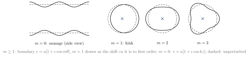
vaft.diagram.cylindrical_mode_morphology()The poloidal mode number as a shape: sausage, kink, and higher helical distortions.
vaft.diagram.cylindrical_mode_morphology(*, labels=True)Show source vaft/diagram/_cylindrical_modes.py, lines 156–195
def cylindrical_mode_morphology(*, labels: bool = True) -> Diagram:
    r"""The poloidal mode number as a shape: sausage, kink, and higher helical distortions.

    $m = 0$ from the side, the radius modulated along $z$; $m = 1, 2, 3$ as
    cross-sections of the boundary $r = a[1 + \epsilon\cos m\theta]$ ($m = 1$
    drawn as the rigid shift it is to first order). Dashed: the unperturbed
    column. Amplitudes are exaggerated.
    """
    labels = _check_labels(labels)
    a, eps = 1.2, 0.18
    items: List = []
    z = np.linspace(0.0, 5.0, 201)
    r0 = a * (1.0 + eps * np.cos(2.0 * math.pi * z / 2.5))
    for sign in (1, -1):
        items += [Polyline.of(np.stack([z, sign * r0], -1), "lcfs", role="mode:0"),
                  Polyline.of(np.stack([z, np.full_like(z, sign * a)], -1), "approx", role="unperturbed")]
    t = np.linspace(0.0, 2.0 * math.pi, 241)
    shapes, centres = {}, {}
    for k, m in enumerate((1, 2, 3)):
        cx = 7.8 + 3.4 * k
        centres[m] = cx
        if m == 1:
            pts = np.stack([cx + eps * a + a * np.cos(t), a * np.sin(t)], -1)
        else:
            r = a * (1.0 + eps * np.cos(m * t))
            pts = np.stack([cx + r * np.cos(t), r * np.sin(t)], -1)
        shapes[m] = pts
        items += [Polyline.of(pts, "lcfs", role=f"mode:{m}", closed=True),
                  Polyline.of(np.stack([cx + a * np.cos(t), a * np.sin(t)], -1), "approx", role="unperturbed",
                              closed=True),
                  Marker((cx, 0.0), "x", "xpoint", role="axis")]
    if labels:
        for text, x in (("$m = 0$: sausage (side view)", 2.5), ("$m = 1$: kink", 7.8), ("$m = 2$", 11.2),
                        ("$m = 3$", 14.6)):
            items.append(Label((x, -a - 0.6), text, "small label", anchor="north", role="title"))
        items.append(_note("$m \\ge 1$: boundary $r = a[1 + \\epsilon\\cos m\\theta]$, $m = 1$ drawn as the shift "
                           "$\\epsilon a$ it is to first order; $m = 0$: $r = a[1 + \\epsilon\\cos kz]$; dashed: "
                           "unperturbed", 8.0, -a - 1.3))
    return Diagram("cylindrical_mode_morphology", Scene(tuple(items)),
                   model={"shapes": shapes, "centres": centres, "epsilon": eps, "a": a, "sausage": r0})
Formats .svg .tex .pdf the SVG above is committed; build the others locally
import vaft.diagram

d = vaft.diagram.cylindrical_mode_morphology()
d.tikz  # the TikZ document as text
d.save("cylindrical_mode_morphology.svg")  # rendered vector image, the canonical artifact; needs latex, dvisvgm
d.save("cylindrical_mode_morphology.tex")  # the complete TikZ document, the text source
d.save("cylindrical_mode_morphology.pdf")  # vector PDF; needs pdflatex
internal_external_kink
1 asset
source
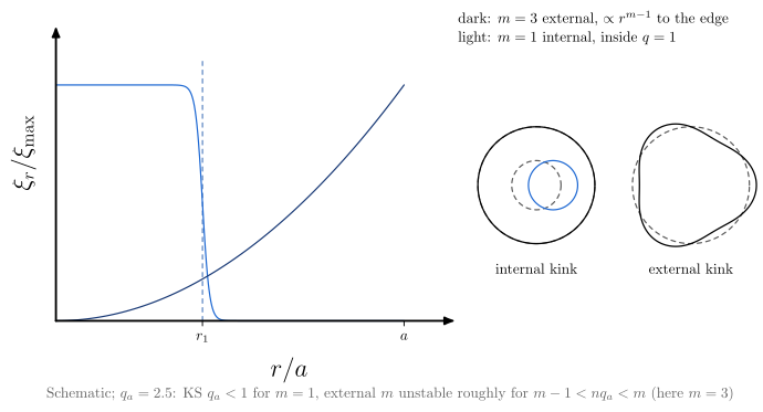
vaft.diagram.internal_external_kink()Internal kink: displacement inside $q = 1$; external kink: displacement reaching the boundary.
vaft.diagram.internal_external_kink(*, labels=True)Show source vaft/diagram/_cylindrical_modes.py, lines 198–253
def internal_external_kink(*, labels: bool = True) -> Diagram:
    r"""Internal kink: displacement inside $q = 1$; external kink: displacement reaching the boundary.

    Left, schematic radial displacements: the $m = 1$ internal kink is a
    rigid shift of the core inside the $q = 1$ radius $r_1$ of a profile with
    $q_0 < 1$ (``peaked_current_safety_factor``, $\nu = 2$, $q_a = 2.5$); an
    $m = 3$ external kink -- $q_a$ just below $m/n$, no $q = 3$ surface inside --
    grows as $r^{m-1}$ up to the edge, where it moves the boundary. Right, the
    matching cross-sections. Kruskal--Shafranov ($q_a < 1$ for $m = 1$; roughly
    $m - 1 < nq_a < m$ for an external $m$ on a flat current) is a heuristic,
    not an exact boundary.
    """
    labels = _check_labels(labels)
    nu, q_a = 2.0, 2.5
    r1 = _root(lambda xx: float(peaked_current_safety_factor(xx, q_a, nu)) - 1.0, 0.0, 1.0)
    x = np.linspace(0.0, 1.0, 401)
    internal = 0.5 * (1.0 - np.tanh((x - r1) / 0.02))
    external = x ** (3 - 1)  # m = 3: q_a = 2.5 < 3 with no q = 3 surface inside, the external-kink window
    chart = Chart(x_range=(0.0, 1.08), y_range=(0.0, 1.15))
    chart.curves.update({"internal": np.stack([x, internal], -1), "external": np.stack([x, external], -1),
                         "q1": np.array([[r1, 0.0], [r1, 1.1]])})
    chart.parameters.update({"r1": r1, "nu": nu, "q_a": q_a})
    scene = render_chart(chart, x_label="$r/a$", y_label="$\\xi_r/\\xi_\\mathrm{max}$",
                         curve_styles={"q1": "rational", "internal": "orbit ion", "external": "orbit electron"},
                         region_text={}, x_ticks=(r1, 1.0), x_tick_text=("$r_1$", "$a$"))
    items: List = list(scene.items)
    t = np.linspace(0.0, 2.0 * math.pi, 241)
    R = 1.4
    for k, (name, cx) in enumerate((("internal", CHART_WIDTH + 2.5), ("external", CHART_WIDTH + 6.2))):
        cy = 0.5 * CHART_HEIGHT
        items.append(Polyline.of(np.stack([cx + R * np.cos(t), cy + R * np.sin(t)], -1), "approx",
                                 role="unperturbed", closed=True))
        if name == "internal":
            items += [Polyline.of(np.stack([cx + R * np.cos(t), cy + R * np.sin(t)], -1), "lcfs",
                                  role="boundary:internal", closed=True),
                      Polyline.of(np.stack([cx + R * r1 * np.cos(t), cy + R * r1 * np.sin(t)], -1),
                                  "approx", role="unperturbed", closed=True),
                      Polyline.of(np.stack([cx + 0.4 + R * r1 * np.cos(t), cy + R * r1 * np.sin(t)], -1),
                                  "orbit ion", role="core:internal", closed=True)]
        else:
            r = R * (1.0 + 0.12 * np.cos(3 * t))
            items.append(Polyline.of(np.stack([cx + r * np.cos(t), cy + r * np.sin(t)], -1), "lcfs",
                                     role="boundary:external", closed=True))
        if labels:
            items.append(Label((cx, cy - R - 0.35), f"{name} kink", "small label", anchor="north", role="title"))
    if labels:
        items += [
            Label((CHART_WIDTH + 0.5, CHART_HEIGHT), "light: $m = 1$ internal, inside $q = 1$", "small label",
                  anchor="south west", role="internal"),
            Label((CHART_WIDTH + 0.5, CHART_HEIGHT + 0.45), "dark: $m = 3$ external, $\\propto r^{m-1}$ to the edge",
                  "small label", anchor="south west", role="external"),
            _note("Schematic; $q_a = 2.5$: KS $q_a < 1$ for $m = 1$, external $m$ unstable roughly for "
                  "$m - 1 < nq_a < m$ (here $m = 3$)",
                  0.5 * (CHART_WIDTH + 7.0), -1.45),
        ]
    return Diagram("internal_external_kink", Scene(tuple(items)), model=chart)
Formats .svg .tex .pdf the SVG above is committed; build the others locally
import vaft.diagram

d = vaft.diagram.internal_external_kink()
d.tikz  # the TikZ document as text
d.save("internal_external_kink.svg")  # rendered vector image, the canonical artifact; needs latex, dvisvgm
d.save("internal_external_kink.tex")  # the complete TikZ document, the text source
d.save("internal_external_kink.pdf")  # vector PDF; needs pdflatex
Formula functions referenced:
geometry.peaked_current_safety_factor
plasma_vacuum_wall
1 asset
source
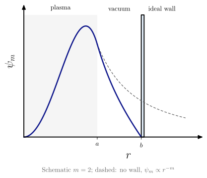
vaft.diagram.plasma_vacuum_wall()One harmonic across plasma, vacuum and an ideal conducting wall.
vaft.diagram.plasma_vacuum_wall(m=2, *, labels=True)Show source vaft/diagram/_cylindrical_modes.py, lines 261–309
def plasma_vacuum_wall(m: int = 2, *, labels: bool = True) -> Diagram:
    r"""One harmonic across plasma, vacuum and an ideal conducting wall.

    Schematic $\psi_m(r)$: regular inside the plasma ($c_1r^m + c_2r^{m+2}$), the vacuum solution $Ar^m + Br^{-m}$ outside, matched to it in value
    and slope at $r = a$ (no edge surface current), and
    $\psi_m(b) = 0$ on an ideal wall at $r = b = 1.6a$; dashed, the same with
    no wall ($\propto r^{-m}$). The problems of external kinks, resistive wall
    modes and tearing outer regions all match such pieces.
    """
    if isinstance(m, bool) or not isinstance(m, (int, np.integer)) or not 1 <= m <= 5:
        raise ValueError(f"m must be an integer from 1 to 5, not {m!r}")
    labels = _check_labels(labels)
    a, b = 1.0, 1.6
    r_in = np.linspace(0.0, a, 201)
    r_out = np.linspace(a, b, 121)
    r_free = np.linspace(a, 2.2, 161)
    A, B = np.linalg.solve([[a ** m, a ** -m], [b ** m, b ** -m]], [1.0, 0.0])
    wall = A * r_out ** m + B * r_out ** -m
    # interior regular at the axis (~ r^m) and matched to the vacuum in value and slope at a: no
    # surface current at the edge, so no kink in psi there
    slope_a = m * A * a ** (m - 1) - m * B * a ** (-m - 1)
    c = np.linalg.solve([[a ** m, a ** (m + 2)], [m * a ** (m - 1), (m + 2) * a ** (m + 1)]], [1.0, slope_a])
    inside = c[0] * r_in ** m + c[1] * r_in ** (m + 2)
    free = (r_free / a) ** -m
    chart = Chart(x_range=(0.0, 2.3), y_range=(0.0, 1.1 * float(inside.max())))
    chart.curves.update({"plasma": np.stack([r_in, inside], -1), "vacuum_wall": np.stack([r_out, wall], -1),
                         "vacuum_free": np.stack([r_free, free], -1)})
    chart.parameters.update({"m": m, "a": a, "b": b, "A": A, "B": B, "interior": c})
    scene = render_chart(chart, x_label="$r$", y_label="$\\psi_m$",
                         curve_styles={"vacuum_free": "approx", "plasma": "boundary", "vacuum_wall": "boundary"},
                         region_text={}, x_ticks=(a, b), x_tick_text=("$a$", "$b$"))
    items: List = []
    x_a = float(chart.to_cm(np.array([a, 0.0]))[0])
    x_b = float(chart.to_cm(np.array([b, 0.0]))[0])
    items += [Polyline.of([(0.0, 0.0), (x_a, 0.0), (x_a, CHART_HEIGHT), (0.0, CHART_HEIGHT)], "concept band",
                          role="region:plasma", closed=True),
              Polyline.of([(x_b, 0.0), (x_b + 0.15, 0.0), (x_b + 0.15, CHART_HEIGHT), (x_b, CHART_HEIGHT)], "section fill",
                          role="region:wall", closed=True)]
    items += list(scene.items)
    if labels:
        items += [
            Label((0.5 * x_a, CHART_HEIGHT + 0.1), "plasma", "small label", anchor="south", role="region:plasma"),
            Label((0.5 * (x_a + x_b), CHART_HEIGHT + 0.1), "vacuum", "small label", anchor="south",
                  role="region:vacuum"),
            Label((x_b + 0.25, CHART_HEIGHT + 0.1), "ideal wall", "small label", anchor="south west",
                  role="region:wall"),
            _note(f"Schematic $m = {m}$; dashed: no wall, $\\psi_m \\propto r^{{-m}}$", CHART_WIDTH / 2, -1.45),
        ]
    return Diagram("plasma_vacuum_wall", Scene(tuple(items)), model=chart)
Formats .svg .tex .pdf the SVG above is committed; build the others locally
import vaft.diagram

d = vaft.diagram.plasma_vacuum_wall()
d.tikz  # the TikZ document as text
d.save("plasma_vacuum_wall.svg")  # rendered vector image, the canonical artifact; needs latex, dvisvgm
d.save("plasma_vacuum_wall.tex")  # the complete TikZ document, the text source
d.save("plasma_vacuum_wall.pdf")  # vector PDF; needs pdflatex
cylindrical_tearing_outer
1 asset
source
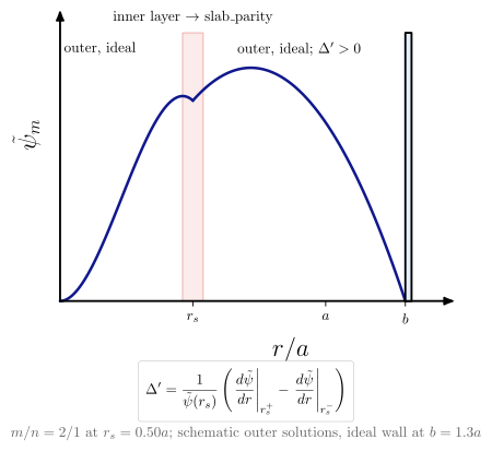
vaft.diagram.cylindrical_tearing_outer()The outer tearing solution of one rational surface on the cylinder, and where the inner layer takes over.
vaft.diagram.cylindrical_tearing_outer(m=2, n=1, *, labels=True)Show source vaft/diagram/_cylindrical_modes.py, lines 312–369
def cylindrical_tearing_outer(m: int = 2, n: int = 1, *, labels: bool = True) -> Diagram:
    r"""The outer tearing solution of one rational surface on the cylinder, and where the inner layer takes over.

    $r_s$ from $q(r_s) = m/n$ (``peaked_current_safety_factor``, $\nu = 1$,
    $q_a = 3.5$); schematic outer solutions $\propto r^m$ near the axis and
    vanishing at an ideal wall $b = 1.3a$, meeting at $\psi_m(r_s)$ with a
    slope jump, whose $\Delta'$ is ``delta_prime_from_outer_derivatives`` of
    the drawn slopes. The shaded layer at $r_s$ is the non-ideal region of
    ``slab_parity``; $\Delta'$ belongs to the outer, ideal cylindrical problem.
    """
    for name, v in (("m", m), ("n", n)):
        if isinstance(v, bool) or not isinstance(v, (int, np.integer)) or v <= 0:
            raise ValueError(f"{name} must be a positive integer mode number, not {v!r}")
    q0 = _QA / (_NU + 1.0)
    if not q0 < m / n < _QA:
        raise ValueError(f"m/n = {m}/{n} has no rational surface in this profile (q from {q0:g} to {_QA:g})")
    labels = _check_labels(labels)
    rs = _root(lambda xx: float(peaked_current_safety_factor(xx, _QA, _NU)) - m / n, 0.0, 1.0)
    b = 1.3
    # left: psi = c1 r^m + c2 r^(m+1), psi(rs) = 1, slope s_minus; right: quadratic in (b - r), psi(b) = 0
    s_minus, s_plus = -0.6 / rs, 1.2 / (b - rs)
    c = np.linalg.solve([[rs ** m, rs ** (m + 1)], [m * rs ** (m - 1), (m + 1) * rs ** m]], [1.0, s_minus])
    u = b - rs
    d = np.linalg.solve([[u, u * u], [1.0, 2.0 * u]], [1.0, -s_plus])
    r_left = np.linspace(0.0, rs, 201)
    r_right = np.linspace(rs, b, 201)
    left = c[0] * r_left ** m + c[1] * r_left ** (m + 1)
    right = d[0] * (b - r_right) + d[1] * (b - r_right) ** 2
    value = delta_prime_from_outer_derivatives(1.0, s_minus, s_plus)
    top = 1.15 * float(max(left.max(), right.max()))
    chart = Chart(x_range=(0.0, 1.4), y_range=(0.0, top))
    chart.curves.update({"outer_left": np.stack([r_left, left], -1), "outer_right": np.stack([r_right, right], -1)})
    chart.parameters.update({"m": m, "n": n, "r_s": rs, "b": b, "dpsi_dr_minus": s_minus, "dpsi_dr_plus": s_plus,
                             "delta_prime": value})
    scene = render_chart(chart, x_label="$r/a$", y_label="$\\tilde\\psi_m$",
                         curve_styles={"outer_left": "outer solution", "outer_right": "outer solution"},
                         region_text={}, x_ticks=(rs, 1.0, b), x_tick_text=("$r_s$", "$a$", "$b$"))
    xs = float(chart.to_cm(np.array([rs, 0.0]))[0])
    half = 0.25
    items: List = [Polyline.of([(xs - half, 0.0), (xs + half, 0.0), (xs + half, CHART_HEIGHT), (xs - half, CHART_HEIGHT)],
                               "layer", role="inner_layer", closed=True)]
    items += list(scene.items)
    x_b = float(chart.to_cm(np.array([b, 0.0]))[0])
    items.append(Polyline.of([(x_b, 0.0), (x_b + 0.15, 0.0), (x_b + 0.15, CHART_HEIGHT), (x_b, CHART_HEIGHT)],
                             "section fill", role="wall", closed=True))
    if labels:
        items += [
            Label((xs, CHART_HEIGHT + 0.1), "inner layer $\\to$ slab\\_parity", "small label", anchor="south",
                  role="inner_layer"),
            Label((0.3 * xs, CHART_HEIGHT - 0.1), "outer, ideal", "small label", anchor="north", role="outer"),
            Label((0.5 * (xs + x_b), CHART_HEIGHT - 0.1), f"outer, ideal; $\\Delta' {'>' if value > 0 else '<'} 0$",
                  "small label", anchor="north", role="delta_prime"),
            Label((CHART_WIDTH / 2, -1.45), f"$\\displaystyle {formula_equation(delta_prime_from_outer_derivatives)}$",
                  "formula box", anchor="north", role="equations"),
            _note(f"$m/n = {m}/{n}$ at $r_s = {rs:.2f}a$; schematic outer solutions, ideal wall at $b = {b:g}a$",
                  CHART_WIDTH / 2, -2.9),
        ]
    return Diagram("cylindrical_tearing_outer", Scene(tuple(items)), model=chart)
Formats .svg .tex .pdf the SVG above is committed; build the others locally
import vaft.diagram

d = vaft.diagram.cylindrical_tearing_outer()
d.tikz  # the TikZ document as text
d.save("cylindrical_tearing_outer.svg")  # rendered vector image, the canonical artifact; needs latex, dvisvgm
d.save("cylindrical_tearing_outer.tex")  # the complete TikZ document, the text source
d.save("cylindrical_tearing_outer.pdf")  # vector PDF; needs pdflatex
Formula functions referenced:
geometry.peaked_current_safety_factor, stability.delta_prime_from_outer_derivatives
Current-profile and safety-factor topology: shapes, l_i, q landmarks, rational surfaces
Module vaft.diagram._equilibrium_profiles
current_profile_shapes
1 asset
source
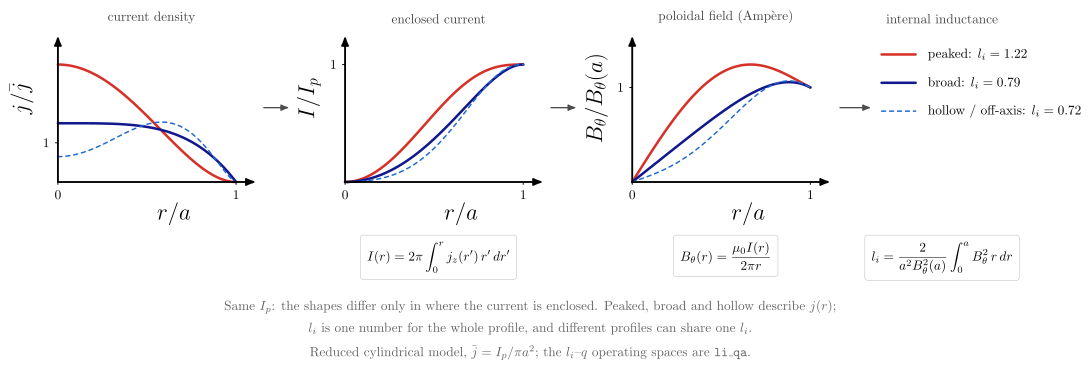
vaft.diagram.current_profile_shapes()Current-profile shapes at the same $I_p$: $j(r) \to I(r) \to B_\theta(r) \to l_i$.
vaft.diagram.current_profile_shapes(profiles=('peaked', 'broad', 'hollow'), *, labels=True)Show source vaft/diagram/_equilibrium_profiles.py, lines 146–216
def current_profile_shapes(profiles: Sequence[str] = ("peaked", "broad", "hollow"), *,
                           labels: bool = True) -> Diagram:
    r"""Current-profile shapes at the same $I_p$: $j(r) \to I(r) \to B_\theta(r) \to l_i$.

    Peaked $j \propto (1 - x^2)^2$, broad $1 - x^4$ and hollow (off-axis)
    $(0.1 + x^2)(1 - x^2)^{3/2}$ over $x = r/a$, each normalized to the same
    total current, so they differ only in where the current is enclosed:
    ``cylindrical_enclosed_current`` gives $I(r)$, Ampère
    (``cylindrical_poloidal_field``) $B_\theta(r)$, and
    ``cylindrical_internal_inductance`` $l_i$. The shapes are of the current
    density; $l_i$ is one number for the whole $I(r)$ and is not itself
    peaked or hollow. A more centrally enclosed current tends to a larger
    $l_i$, but different profiles can share one $l_i$. Reduced cylindrical
    model; the $l_i$-$q$ operating spaces are ``li_qa``.
    """
    profiles = _check_names(profiles, tuple(_CURRENTS), "profiles")
    labels = _check_labels(labels)
    models = {p: _cylinder(p) for p in profiles}
    x = models[profiles[0]]["x"]
    panels = (("j", "$j/\\bar j$", "current density", None),
              ("I", "$I/I_p$", "enclosed current", cylindrical_enclosed_current),
              ("B_theta", "$B_\\theta/B_\\theta(a)$", "poloidal field (Ampère)", cylindrical_poloidal_field))
    step = 7.6
    items: List = []
    charts: Dict[str, Chart] = {}
    for k, (key, y_label, title, formula) in enumerate(panels):
        top = 1.15 * max(float(np.max(m[key])) for m in models.values())
        chart = Chart(x_range=(0.0, 1.05), y_range=(0.0, top))
        for p, m in models.items():
            chart.curves[p] = np.stack([x, m[key]], -1)
        charts[key] = chart
        items += _panel(chart, (k * step, 0.0), x_label="$r/a$", y_label=y_label,
                        curve_styles={p: _STYLE[p] for p in profiles}, region_text={}, x_ticks=(0.0, 1.0),
                        y_ticks=(1.0,), y_tick_text=("$1$",))
        if labels:
            items.append(Label((k * step + _PANEL * 0.5 * CHART_WIDTH, _PANEL * CHART_HEIGHT + 0.5), title,
                               "subtitle", anchor="south", role="title"))
            if formula is not None:
                items.append(Label((k * step + _PANEL * 0.5 * CHART_WIDTH, -1.4),
                                   f"$\\displaystyle {formula_equation(formula)}$", "formula box", anchor="north",
                                   role="equations"))
        if k:
            y = _PANEL * CHART_HEIGHT * 0.55
            items.append(Arrow(((k - 1) * step + _PANEL * CHART_WIDTH + 0.5, y), (k * step - 1.45, y), "connector",
                               role="chain"))
    # the l_i column: one value per profile, keyed by its line
    x0 = 3 * step - 1.0
    y_top = _PANEL * CHART_HEIGHT - 0.2
    items.append(Arrow((2 * step + _PANEL * CHART_WIDTH + 0.55, _PANEL * CHART_HEIGHT * 0.55),
                       (x0 - 0.25, _PANEL * CHART_HEIGHT * 0.55), "connector", role="chain"))
    for i, p in enumerate(profiles):
        y = y_top - 0.75 * i
        items.append(Polyline.of([(x0, y), (x0 + 0.9, y)], _STYLE[p], role=f"legend:{p}"))
        if labels:
            items.append(Label((x0 + 1.1, y), f"{_CURRENT_TEXT[p]}: $l_i = {models[p]['l_i']:.2f}$", "small label",
                               anchor="west", role=f"l_i:{p}"))
    if labels:
        items += [
            Label((x0 + 1.6, _PANEL * CHART_HEIGHT + 0.5), "internal inductance", "subtitle", anchor="south",
                  role="title"),
            Label((x0 + 1.6, -1.4), f"$\\displaystyle {formula_equation(cylindrical_internal_inductance)}$",
                  "formula box", anchor="north", role="equations"),
            _note("Same $I_p$: the shapes differ only in where the current is enclosed. Peaked, broad and hollow "
                  "describe $j(r)$;", 12.5, -3.0),
            _note("$l_i$ is one number for the whole profile, and different profiles can share one $l_i$.",
                  12.5, -3.6),
            _note("Reduced cylindrical model, $\\bar j = I_p/\\pi a^2$; the $l_i$--$q$ operating spaces are "
                  "\\texttt{li\\_qa}.", 12.5, -4.2),
        ]
    model = {"profiles": models, "charts": charts}
    return Diagram("current_profile_shapes", Scene(tuple(items)), model=model)
Formats .svg .tex .pdf the SVG above is committed; build the others locally
import vaft.diagram

d = vaft.diagram.current_profile_shapes()
d.tikz  # the TikZ document as text
d.save("current_profile_shapes.svg")  # rendered vector image, the canonical artifact; needs latex, dvisvgm
d.save("current_profile_shapes.tex")  # the complete TikZ document, the text source
d.save("current_profile_shapes.pdf")  # vector PDF; needs pdflatex
Formula functions referenced:
equilibrium.shear_from_r_q, geometry.cylindrical_enclosed_current, geometry.cylindrical_internal_inductance, geometry.cylindrical_poloidal_field, geometry.cylindrical_poloidal_flux, geometry.cylindrical_safety_factor_from_r_B
q_profile_landmarks
2 assets
source
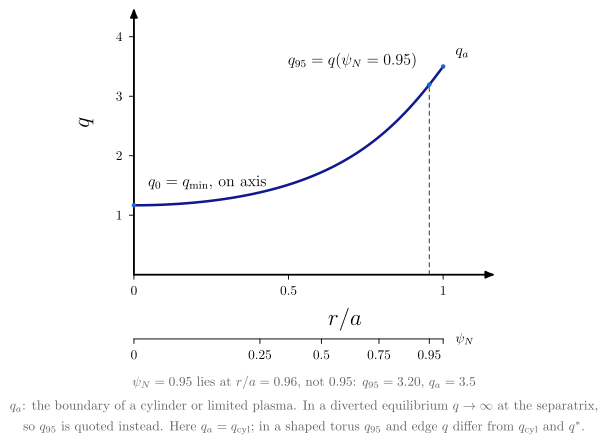
vaft.diagram.q_profile_landmarks(profile='monotonic')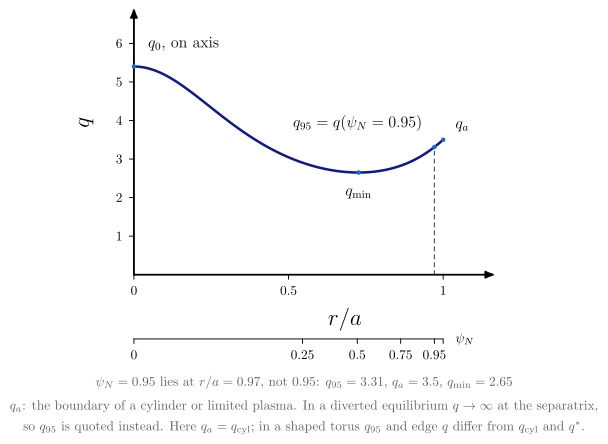
vaft.diagram.q_profile_landmarks(profile='reversed_shear')Where $q_0$, $q_\min$, $q_{95}$ and the edge $q_a$ sit on one safety-factor profile.
vaft.diagram.q_profile_landmarks(profile='monotonic', *, labels=True)Show source vaft/diagram/_equilibrium_profiles.py, lines 224–289
def q_profile_landmarks(profile: str = "monotonic", *, labels: bool = True) -> Diagram:
    r"""Where $q_0$, $q_\min$, $q_{95}$ and the edge $q_a$ sit on one safety-factor profile.

    $q(r/a)$ of the reduced cylinder (``profile="monotonic"``: the peaked
    current; ``"reversed_shear"``: the hollow one), with a second axis giving
    the normalized poloidal flux $\psi_N$ (``cylindrical_poloidal_flux``) at
    each radius. $q_0$ is on axis; $q_\min$ is the minimum, equal to $q_0$
    only for a monotonic $q$; $q_{95} = q(\psi_N = 0.95)$, which is not at
    $r/a = 0.95$; $q_a$ is the boundary value of a cylinder or limited
    plasma -- in a diverted equilibrium $q \to \infty$ at the separatrix,
    which is why $q_{95}$ is quoted. In this cylinder $q_a = q_\mathrm{cyl}$
    by construction; in a shaped, finite-aspect-ratio torus $q_{95}$ and the
    equilibrium edge $q$ differ from $q_\mathrm{cyl}$ and $q^*$.
    """
    profile = _check_name(profile, ("monotonic", "reversed_shear"), "profile")
    labels = _check_labels(labels)
    m = _cylinder(_TOPOLOGY[profile])
    x, q = m["x"], m["q"]
    x95, q95 = _x_at_psi_n(m, 0.95), _q_at_psi_n(m, 0.95)
    top = 1.18 * max(float(q.max()), m["q_a"])
    chart = Chart(x_range=(0.0, 1.1), y_range=(0.0, top))
    chart.curves["q"] = np.stack([x, q], -1)
    chart.curves["drop_95"] = np.array([[x95, 0.0], [x95, q95]])
    chart.points.update({"q0": (0.0, m["q0"]), "q_min": (m["x_min"], m["q_min"]), "q95": (x95, q95),
                         "q_a": (1.0, m["q_a"])})
    chart.parameters.update({"profile": profile, "x95": x95, "q95": q95, "q0": m["q0"], "q_min": m["q_min"],
                             "x_min": m["x_min"], "q_a": m["q_a"]})
    scene = render_chart(chart, x_label="$r/a$", y_label="$q$", curve_styles={"q": "boundary", "drop_95": "approx"},
                         region_text={}, x_ticks=(0.0, 0.5, 1.0), y_ticks=tuple(range(1, int(top) + 1)))
    items: List = list(scene.items)
    # the psi_N axis under the r/a ticks: where each flux fraction is in radius
    y_axis = -1.7
    items.append(Polyline.of([(0.0, y_axis), tuple(chart.to_cm(np.array([1.0, 0.0])) + [0.0, y_axis])],
                             "tick", role="psi_n_axis"))
    for value in (0.0, 0.25, 0.5, 0.75, 0.95, 1.0):
        cx = float(chart.to_cm(np.array([_x_at_psi_n(m, value), 0.0]))[0])
        items.append(Polyline.of([(cx, y_axis), (cx, y_axis - 0.12)], "tick", role="psi_n_axis"))
        if labels and value != 1.0:
            items.append(Label((cx, y_axis - 0.18), f"${value:g}$", "ticklabel", anchor="north",
                               role="psi_n_axis"))
    for name in ("q0", "q95", "q_a") + (("q_min",) if profile == "reversed_shear" else ()):
        items.append(Marker(tuple(chart.to_cm(chart.points[name])), "o", "opoint", role=name))
    if labels:
        right = float(chart.to_cm(np.array([1.0, 0.0]))[0])
        items.append(Label((right + 0.2, y_axis), "$\\psi_N$", "ticklabel", anchor="west", role="psi_n_axis"))
        p0 = chart.to_cm(chart.points["q0"])
        q0_text = ("$q_0 = q_{\\min}$" if profile == "monotonic" else "$q_0$") + ", on axis"
        items.append(Label((p0[0] + 0.25, p0[1] + 0.3), q0_text, "label", anchor="south west", role="q0"))
        if profile == "reversed_shear":
            pm = chart.to_cm(chart.points["q_min"])
            items.append(Label((pm[0], pm[1] - 0.3), "$q_{\\min}$", "label", anchor="north", role="q_min"))
        p95 = chart.to_cm(chart.points["q95"])
        items.append(Label((p95[0] - 0.2, p95[1] + 0.3), "$q_{95} = q(\\psi_N = 0.95)$", "label",
                           anchor="south east", role="q95"))
        pa = chart.to_cm(chart.points["q_a"])
        items.append(Label((pa[0] + 0.2, pa[1] + 0.1), "$q_a$", "label", anchor="south west", role="q_a"))
        items += [
            _note(f"$\\psi_N = 0.95$ lies at $r/a = {x95:.2f}$, not $0.95$: $q_{{95}} = {q95:.2f}$, "
                  f"$q_a = {m['q_a']:g}$" + (f", $q_{{\\min}} = {m['q_min']:.2f}$" if profile == "reversed_shear"
                                             else ""), CHART_WIDTH / 2, -2.55),
            _note("$q_a$: the boundary of a cylinder or limited plasma. In a diverted equilibrium "
                  "$q \\to \\infty$ at the separatrix,", CHART_WIDTH / 2, -3.2),
            _note("so $q_{95}$ is quoted instead. Here $q_a = q_\\mathrm{cyl}$; in a shaped torus $q_{95}$ and "
                  "edge $q$ differ from $q_\\mathrm{cyl}$ and $q^*$.", CHART_WIDTH / 2, -3.75),
        ]
    return Diagram("q_profile_landmarks", Scene(tuple(items)), model=chart)
Formats .svg .tex .pdf the SVG above is committed; build the others locally
import vaft.diagram

d = vaft.diagram.q_profile_landmarks(profile='monotonic')
d.tikz  # the TikZ document as text
d.save("q_profile_landmarks_monotonic.svg")  # rendered vector image, the canonical artifact; needs latex, dvisvgm
d.save("q_profile_landmarks_monotonic.tex")  # the complete TikZ document, the text source
d.save("q_profile_landmarks_monotonic.pdf")  # vector PDF; needs pdflatex
Formula functions referenced:
equilibrium.shear_from_r_q, geometry.cylindrical_enclosed_current, geometry.cylindrical_internal_inductance, geometry.cylindrical_poloidal_field, geometry.cylindrical_poloidal_flux, geometry.cylindrical_safety_factor_from_r_B
q_profile_topologies
1 asset
source
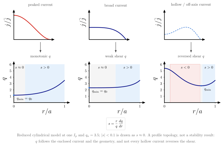
vaft.diagram.q_profile_topologies()Monotonic, weak-shear and reversed-shear $q$, each from its current shape, with the sign of the shear.
vaft.diagram.q_profile_topologies(profiles=('monotonic', 'weak_shear', 'reversed_shear'), *, labels=True)Show source vaft/diagram/_equilibrium_profiles.py, lines 312–379
def q_profile_topologies(profiles: Sequence[str] = ("monotonic", "weak_shear", "reversed_shear"), *,
                         labels: bool = True) -> Diagram:
    r"""Monotonic, weak-shear and reversed-shear $q$, each from its current shape, with the sign of the shear.

    Columns of the reduced cylinder at one $I_p$ and $q_a$: the peaked
    current gives a monotonic $q$ with $q_\min = q_0$; the broad current a
    wide core where $q$ is nearly flat; the hollow current a $q$ whose
    minimum is off axis, with $s < 0$ inside $q_\min$. $s = (r/q)\,dq/dr$
    is ``shear_from_r_q``, and $|s| < 0.1$ is drawn as $s \approx 0$. Every
    $q$ has $s \to 0$ on axis, so each column carries a narrow
    $s \approx 0$ band there; what singles out the broad current is the
    width of its flat core, not the band itself. This is a profile
    topology, not a stability diagram; $q$ depends on the enclosed current
    and the geometry, and not every hollow current reverses the shear.
    """
    profiles = _check_names(profiles, tuple(_TOPOLOGY), "profiles")
    labels = _check_labels(labels)
    models = {p: _cylinder(_TOPOLOGY[p]) for p in profiles}
    q_top = 1.12 * max(float(m["q"].max()) for m in models.values())
    j_top = 1.15 * max(float(m["j"].max()) for m in models.values())
    step = 7.0
    j_base = _PANEL * CHART_HEIGHT + 2.3
    items: List = []
    runs_of: Dict[str, List] = {}
    for k, p in enumerate(profiles):
        m = models[p]
        x0 = k * step
        jc = Chart(x_range=(0.0, 1.05), y_range=(0.0, j_top))
        jc.curves["j"] = np.stack([m["x"], m["j"]], -1)
        items += _panel(jc, (x0, j_base), scale=0.4, x_label="", y_label="$j/\\bar j$",
                        curve_styles={"j": _STYLE[m["shape"]]}, region_text={})
        qc = Chart(x_range=(0.0, 1.05), y_range=(0.0, q_top))
        qc.curves["q"] = np.stack([m["x"], m["q"]], -1)
        runs = _shear_runs(m["x"], m["s"])
        runs_of[p] = runs
        for sign, a, b in runs:
            (xa, _), (xb, _) = _to_panel(qc, (a, 0.0), (x0, 0.0)), _to_panel(qc, (b, 0.0), (x0, 0.0))
            items.append(Polyline.of([(xa, 0.0), (xb, 0.0), (xb, _PANEL * CHART_HEIGHT), (xa, _PANEL * CHART_HEIGHT)],
                                     _SHEAR_FILL[sign], role=f"shear:{sign}", closed=True))
            if labels and xb - xa > 0.7:
                items.append(Label((0.5 * (xa + xb), _PANEL * CHART_HEIGHT - 0.05), _SHEAR_TEXT[sign],
                                   "small label", anchor="north", role=f"shear:{sign}"))
        items += _panel(qc, (x0, 0.0), x_label="$r/a$", y_label="$q$", curve_styles={"q": "boundary"},
                        region_text={}, x_ticks=(0.0, 1.0), y_ticks=tuple(range(1, int(q_top) + 1)))
        at = _to_panel(qc, (m["x_min"], m["q_min"]), (x0, 0.0))
        items.append(Marker(at, "o", "opoint", role="q_min"))
        if labels:
            text = "$q_{\\min} = q_0$" if m["x_min"] < 0.02 else "$q_{\\min}$"
            items.append(Label((at[0] + 0.15, at[1] - 0.12), text, "small label", anchor="north west", role="q_min"))
            items.append(Label((x0 + _PANEL * 0.5 * CHART_WIDTH, j_base + 0.4 * CHART_HEIGHT + 0.35),
                               f"{_CURRENT_TEXT[m['shape']]} current", "subtitle", anchor="south", role="title"))
            items.append(Arrow((x0 + _PANEL * 0.5 * CHART_WIDTH, j_base - 0.25),
                               (x0 + _PANEL * 0.5 * CHART_WIDTH, _PANEL * CHART_HEIGHT + 1.05), "connector",
                               role="chain"))
            items.append(Label((x0 + _PANEL * 0.5 * CHART_WIDTH, _PANEL * CHART_HEIGHT + 0.45),
                               f"{_TOPOLOGY_TEXT[p]} $q$", "subtitle", anchor="south", role="title"))
    if labels:
        mid = 0.5 * ((len(profiles) - 1) * step + _PANEL * CHART_WIDTH)
        items += [
            Label((mid, -1.4), f"$\\displaystyle {formula_equation(shear_from_r_q)}$", "formula box",
                  anchor="north", role="equations"),
            _note(f"Reduced cylindrical model at one $I_p$ and $q_a = {_Q_A:g}$; $|s| < {_WEAK_SHEAR:g}$ is drawn as "
                  "$s \\approx 0$. A profile topology, not a stability result:", mid, -2.75),
            _note("$q$ follows the enclosed current and the geometry, and not every hollow current reverses the "
                  "shear.", mid, -3.35),
        ]
    model = {"profiles": models, "shear_runs": runs_of}
    return Diagram("q_profile_topologies", Scene(tuple(items)), model=model)
Formats .svg .tex .pdf the SVG above is committed; build the others locally
import vaft.diagram

d = vaft.diagram.q_profile_topologies()
d.tikz  # the TikZ document as text
d.save("q_profile_topologies.svg")  # rendered vector image, the canonical artifact; needs latex, dvisvgm
d.save("q_profile_topologies.tex")  # the complete TikZ document, the text source
d.save("q_profile_topologies.pdf")  # vector PDF; needs pdflatex
Formula functions referenced:
equilibrium.shear_from_r_q, geometry.cylindrical_enclosed_current, geometry.cylindrical_internal_inductance, geometry.cylindrical_poloidal_field, geometry.cylindrical_poloidal_flux, geometry.cylindrical_safety_factor_from_r_B
rational_surface_topology
2 assets
source
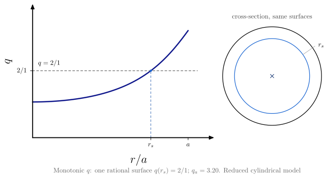
vaft.diagram.rational_surface_topology(profile='monotonic')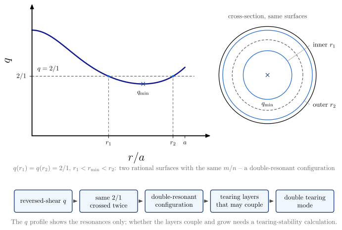
vaft.diagram.rational_surface_topology(profile='reversed_shear')How one $m/n$ meets each $q$ topology: once on a monotonic $q$, twice on a reversed-shear $q$.
vaft.diagram.rational_surface_topology(profile='reversed_shear', m=2, n=1, *, labels=True)Formats .svg .tex .pdf the SVG above is committed; build the others locally
import vaft.diagram

d = vaft.diagram.rational_surface_topology(profile='monotonic')
d.tikz  # the TikZ document as text
d.save("rational_surface_topology_monotonic.svg")  # rendered vector image, the canonical artifact; needs latex, dvisvgm
d.save("rational_surface_topology_monotonic.tex")  # the complete TikZ document, the text source
d.save("rational_surface_topology_monotonic.pdf")  # vector PDF; needs pdflatex
Formula functions referenced:
equilibrium.shear_from_r_q, geometry.cylindrical_enclosed_current, geometry.cylindrical_internal_inductance, geometry.cylindrical_poloidal_field, geometry.cylindrical_poloidal_flux, geometry.cylindrical_safety_factor_from_r_B
Current diffusion and current drive: how $j_\phi(\rho, t)$ and $q(\rho, t)$ evolve
Module vaft.diagram._current_diffusion
current_diffusion
1 asset
source
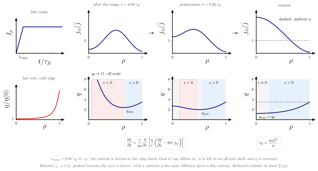
vaft.diagram.current_diffusion()Ohmic current diffusion after a fast ramp: hollow current, reversed shear, relaxation.
vaft.diagram.current_diffusion(*, labels=True)Formats .svg .tex .pdf the SVG above is committed; build the others locally
import vaft.diagram

d = vaft.diagram.current_diffusion()
d.tikz  # the TikZ document as text
d.save("current_diffusion.svg")  # rendered vector image, the canonical artifact; needs latex, dvisvgm
d.save("current_diffusion.tex")  # the complete TikZ document, the text source
d.save("current_diffusion.pdf")  # vector PDF; needs pdflatex
Formula functions referenced:
equilibrium.shear_from_r_q, equilibrium.spitzer_resistivity_from_T_e_Z_eff_ln_Lambda, geometry.cylindrical_current_diffusion_rate, ordering.resistive_diffusion_time
current_drive_profiles
2 assets
source
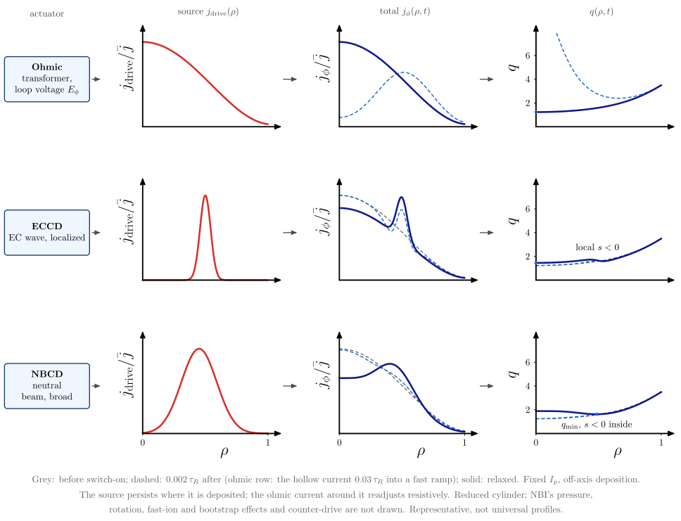
vaft.diagram.current_drive_profiles(deposition='off_axis')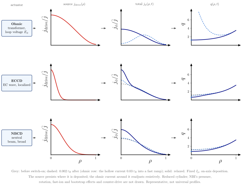
vaft.diagram.current_drive_profiles(deposition='on_axis')Ohmic, ECCD and NBCD: actuator $\to$ source $j_\mathrm{drive}(\rho)$ $\to$ total $j_\phi(\rho, t)$ $\to$ $q(\rho, t)$.
vaft.diagram.current_drive_profiles(deposition='off_axis', *, labels=True)Formats .svg .tex .pdf the SVG above is committed; build the others locally
import vaft.diagram

d = vaft.diagram.current_drive_profiles(deposition='off_axis')
d.tikz  # the TikZ document as text
d.save("current_drive_profiles_off_axis.svg")  # rendered vector image, the canonical artifact; needs latex, dvisvgm
d.save("current_drive_profiles_off_axis.tex")  # the complete TikZ document, the text source
d.save("current_drive_profiles_off_axis.pdf")  # vector PDF; needs pdflatex
Formula functions referenced:
equilibrium.shear_from_r_q, equilibrium.spitzer_resistivity_from_T_e_Z_eff_ln_Lambda, geometry.cylindrical_current_diffusion_rate, ordering.resistive_diffusion_time
Canonical slab field configurations and reconnection topology
Module vaft.diagram._field_configurations
slab_field_configuration
4 assets
source
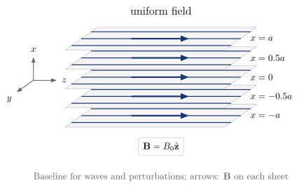
vaft.diagram.slab_field_configuration(kind='uniform')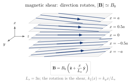
vaft.diagram.slab_field_configuration(kind='sheared')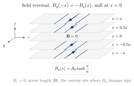
vaft.diagram.slab_field_configuration(kind='reversed')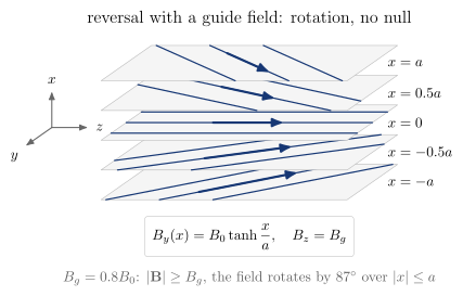
vaft.diagram.slab_field_configuration(kind='guide')Field direction on stacked $x$ = const sheets: uniform, sheared, reversed, guide-field.
vaft.diagram.slab_field_configuration(kind='sheared', *, labels=True)Show source vaft/diagram/_field_configurations.py, lines 108–182
def slab_field_configuration(kind: str = "sheared", *, labels: bool = True) -> Diagram:
    r"""Field direction on stacked $x$ = const sheets: uniform, sheared, reversed, guide-field.

    Five sheets at $x/a = -1, -\tfrac12, 0, \tfrac12, 1$, each carrying field
    lines along its $(B_y, B_z)$ and an arrow whose length is $|\mathbf B|$:
    ``uniform`` $\mathbf B = B_0\hat{\mathbf z}$; ``sheared``
    ``sheared_slab_field`` ($L_s = 3a$), the direction rotates while
    $|\mathbf B| = B_0$ to first order in $x/L_s$ (5 % more at $x = a$); ``reversed`` ``harris_sheet_field``, the
    direction flips and $|\mathbf B| = 0$ at $x = 0$; ``guide`` the same plus
    $B_g\hat{\mathbf z}$ ($B_g = 0.8B_0$), rotating through the sheet without a
    null. Shear is a rotation of the field; reversal is a change of sign of
    one component -- the current sheet of ``current_sheet``.
    """
    if kind not in KINDS:
        raise ValueError(f"kind must be one of {KINDS}, not {kind!r}")
    labels = _check_labels(labels)
    levels = np.array([-1.0, -0.5, 0.0, 0.5, 1.0])
    fields = _field(kind, levels)
    items: List = []
    for x_level, (b_y, b_z) in zip(levels, fields):
        corners = _screen(x_level, [0.0, 0.0, _LY, _LY], [0.0, _LZ, _LZ, 0.0])
        items.append(Polyline.of(corners, "concept band", role=f"sheet:{x_level:g}", closed=True))
        items.append(Polyline.of(corners, "surface", role=f"sheet:{x_level:g}", closed=True))
        mag = math.hypot(b_y, b_z)
        if mag < 1e-9:
            if labels:
                items.append(Label(tuple(_screen(x_level, 0.5 * _LY, 0.5 * _LZ)), "$\\mathbf{B} = 0$",
                                   "small label", role="null"))
            continue
        d = np.array([b_y, b_z]) / mag
        normal = np.array([d[1], -d[0]])
        for off in (-0.9, 0.0, 0.9):
            seg = _clip_line(np.array([0.5 * _LY, 0.5 * _LZ]) + off * normal, d)
            if seg is not None:
                items.append(Polyline.of(_screen(x_level, seg[:, 0], seg[:, 1]), "orbit electron",
                                         role=f"field_line:{x_level:g}"))
        centre = np.array([0.5 * _LY, 0.5 * _LZ])
        half = 1.1 * mag / _B0
        a, b = centre - half * d, centre + half * d
        items.append(Arrow(tuple(_screen(x_level, a[0], a[1])), tuple(_screen(x_level, b[0], b[1])),
                           "field vector", role=f"B:{x_level:g}"))
    if labels:
        for x_level in levels:
            text = {1.0: "$x = a$", -1.0: "$x = -a$", 0.0: "$x = 0$"}.get(float(x_level), f"$x = {x_level:g}a$")
            items.append(Label(tuple(_screen(x_level, 0.5 * _LY, _LZ) + np.array([0.25, 0.0])), text, "small label",
                               anchor="west", role="x_level"))
        # the triad: x up, z along the sheets, y receding
        o = np.array([-1.2 + _OBL[0] * _LY, -1.0 * _SPACING + 0.9])
        items += [Arrow(tuple(o), tuple(o + [0.0, 0.9]), "frame axis arrow", role="triad"),
                  Arrow(tuple(o), tuple(o + [0.9, 0.0]), "frame axis arrow", role="triad"),
                  Arrow(tuple(o), tuple(o + 1.6 * np.array(_OBL)), "frame axis arrow", role="triad"),
                  Label(tuple(o + [0.0, 0.95]), "$x$", "small label", anchor="south", role="triad"),
                  Label(tuple(o + [0.95, 0.0]), "$z$", "small label", anchor="west", role="triad"),
                  Label(tuple(o + 1.7 * np.array(_OBL)), "$y$", "small label", anchor="north east", role="triad")]
        title = {"uniform": "uniform field", "sheared": "magnetic shear: direction rotates, $|\\mathbf{B}| \\simeq B_0$",
                 "reversed": "field reversal: $B_y(-x) = -B_y(x)$, null at $x = 0$",
                 "guide": "reversal with a guide field: rotation, no null"}[kind]
        top = 1.0 * _SPACING + max(0.0, _OBL[1] * _LY)
        items.append(Label((0.5 * (_LZ + _OBL[0] * _LY), top + 0.35), title, "label", anchor="south",
                           role="title"))
        eq = {"uniform": "\\mathbf{B} = B_0\\hat{\\mathbf{z}}",
              "sheared": formula_equation(sheared_slab_field),
              "reversed": formula_equation(harris_sheet_field),
              "guide": formula_equation(harris_sheet_field) + ",\\quad B_z = B_g"}[kind]
        bottom = -1.0 * _SPACING + min(0.0, _OBL[1] * _LY) - 0.4
        items.append(Label((0.5 * (_LZ + _OBL[0] * _LY), bottom), f"$\\displaystyle {eq}$", "formula box",
                           anchor="north", role="equations"))
        note = {"uniform": "Baseline for waves and perturbations; arrows: $\\mathbf{B}$ on each sheet",
                "sheared": f"$L_s = {_LS:g}a$; the rotation is the shear, $k_\\parallel(x) = k_yx/L_s$",
                "reversed": "$B_z = 0$; arrow length $|\\mathbf{B}|$; the current sits where $B_y$ changes sign",
                "guide": f"$B_g = {_BG:g}B_0$: $|\\mathbf{{B}}| \\ge B_g$, the field rotates by "
                         f"${2 * math.degrees(math.atan(_B0 * math.tanh(1.0) / _BG)):.0f}^\\circ$ over $|x| \\le a$"}[kind]
        items.append(_note(note, 0.5 * (_LZ + _OBL[0] * _LY), bottom - 1.2))
    return Diagram(f"slab_field_configuration_{kind}", Scene(tuple(items)),
                   model={"kind": kind, "x": levels, "field": fields})
Formats .svg .tex .pdf the SVG above is committed; build the others locally
import vaft.diagram

d = vaft.diagram.slab_field_configuration(kind='uniform')
d.tikz  # the TikZ document as text
d.save("slab_field_configuration_uniform.svg")  # rendered vector image, the canonical artifact; needs latex, dvisvgm
d.save("slab_field_configuration_uniform.tex")  # the complete TikZ document, the text source
d.save("slab_field_configuration_uniform.pdf")  # vector PDF; needs pdflatex
Formula functions referenced:
geometry.harris_sheet_field, geometry.sheared_slab_field
current_sheet
2 assets
source
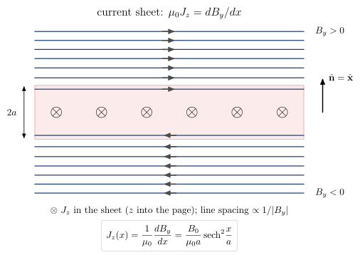
vaft.diagram.current_sheet()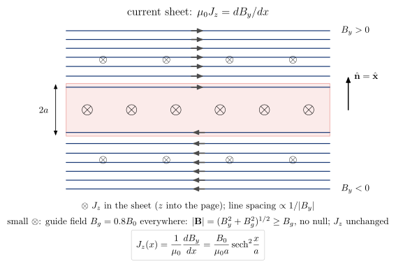
vaft.diagram.current_sheet(guide_field=True)A current sheet seen along the current: reversing field, sheet, normal, thickness, $J_z$.
vaft.diagram.current_sheet(guide_field=False, *, labels=True)Show source vaft/diagram/_field_configurations.py, lines 190–256
def current_sheet(guide_field: bool = False, *, labels: bool = True) -> Diagram:
    r"""A current sheet seen along the current: reversing field, sheet, normal, thickness, $J_z$.

    Field lines of ``harris_sheet_field`` at equal steps of the flux function
    $\psi(x) = B_0a\ln\cosh(x/a)$ ($\mathbf B_\perp = \hat{\mathbf z}\times\nabla\psi$,
    $\psi = -A_z$), so their spacing shows $|B_y|$: dense
    outside, none at the centre. $x$ up is the sheet normal, $y$ across the
    reconnecting direction, $z$ into the page, so the current
    $J_z = \mu_0^{-1}dB_y/dx$ (``harris_sheet_current_density``) of $B_0 > 0$
    is $\otimes$. ``guide_field`` adds $B_g\hat{\mathbf z}$, also $\otimes$ and
    uniform: it leaves this in-plane picture and $J_z$ unchanged and removes
    the null ($|\mathbf B| \ge B_g$).
    """
    if not isinstance(guide_field, bool):
        raise ValueError(f"guide_field must be True or False, not {guide_field!r}")
    labels = _check_labels(labels)
    W, sy = 10.0, 1.0  # sheet length [cm], cm per a
    x_max = 3.0
    flux = lambda x: _B0 * _A * np.log(np.cosh(x / _A))  # noqa: E731 -- psi = -A_z of the Harris field
    steps = np.linspace(0.0, float(flux(x_max)), 8)[1:]
    xs = [_A * math.acosh(math.exp(s / (_B0 * _A))) for s in steps]
    items: List = []
    items.append(Polyline.of([(0.0, -_A * sy), (W, -_A * sy), (W, _A * sy), (0.0, _A * sy)], "layer",
                             role="sheet", closed=True))
    lines = []
    for sign in (1.0, -1.0):
        for x in xs:
            y_cm = sign * x * sy
            items.append(Polyline.of([(0.0, y_cm), (W, y_cm)], "orbit electron", role="field_line"))
            b_y = float(harris_sheet_field(sign * x, _B0, _A))
            mid = 0.5 * W
            direction = 1.0 if b_y > 0 else -1.0
            items.append(Arrow((mid - 0.25 * direction, y_cm), (mid + 0.25 * direction, y_cm), "field arrow",
                               role="field_direction"))
            lines.append((sign * x, b_y))
    for y in np.linspace(0.8, W - 0.8, 6):
        items.append(Label((float(y), 0.0), "$\\otimes$", "legend symbol", role="current"))
    if guide_field:  # B_g along z, into the page like J_z but everywhere: small crossed markers upstream
        for y in np.linspace(1.4, W - 1.4, 4):
            for x in (1.9, -1.9):
                items.append(Label((float(y), x * sy), "$\\otimes$", "charge small", role="guide_field"))
    J0 = float(harris_sheet_current_density(0.0, _B0, _A))
    if labels:
        right = W + 0.3
        items += [
            Arrow((right + 0.4, 0.0), (right + 0.4, 1.3), "vector", role="normal"),
            Label((right + 0.5, 1.3), "$\\hat{\\mathbf{n}} = \\hat{\\mathbf{x}}$", "small label", anchor="west",
                  role="normal"),
            Arrow((-0.4, -_A * sy), (-0.4, _A * sy), "width arrow", role="thickness", both=True),
            Label((-0.55, 0.0), "$2a$", "small label", anchor="east", role="thickness"),
            Label((right, x_max * sy), "$B_y > 0$", "small label", anchor="west", role="upstream"),
            Label((right, -x_max * sy), "$B_y < 0$", "small label", anchor="west", role="upstream"),
            Label((0.5 * W, -x_max * sy - 0.35), "$\\otimes\\ J_z$ in the sheet ($z$ into the page); "
                  "line spacing $\\propto 1/|B_y|$", "small label", anchor="north", role="legend"),
            Label((0.5 * W, x_max * sy + 0.35), "current sheet: $\\mu_0 J_z = dB_y/dx$", "label", anchor="south",
                  role="title"),
        ]
        if guide_field:
            items.append(Label((0.5 * W, -x_max * sy - 0.9), f"small $\\otimes$: guide field $B_g = {_BG:g}B_0$ everywhere: "
                               "$|\\mathbf{B}| = (B_y^2 + B_g^2)^{1/2} \\ge B_g$, no null; $J_z$ unchanged",
                               "small label", anchor="north", role="guide"))
        items.append(Label((0.5 * W, -x_max * sy - (1.55 if guide_field else 1.0)),
                           f"$\\displaystyle {formula_equation(harris_sheet_current_density)}$", "formula box",
                           anchor="north", role="equations"))
    name = "current_sheet_guide_field" if guide_field else "current_sheet"
    return Diagram(name, Scene(tuple(items)), model={"field_lines": lines, "J0": J0, "guide_field": guide_field,
                                                    "B_g": _BG if guide_field else 0.0})
Formats .svg .tex .pdf the SVG above is committed; build the others locally
import vaft.diagram

d = vaft.diagram.current_sheet()
d.tikz  # the TikZ document as text
d.save("current_sheet.svg")  # rendered vector image, the canonical artifact; needs latex, dvisvgm
d.save("current_sheet.tex")  # the complete TikZ document, the text source
d.save("current_sheet.pdf")  # vector PDF; needs pdflatex
Formula functions referenced:
geometry.harris_sheet_current_density, geometry.harris_sheet_field
harris_sheet
1 asset
source
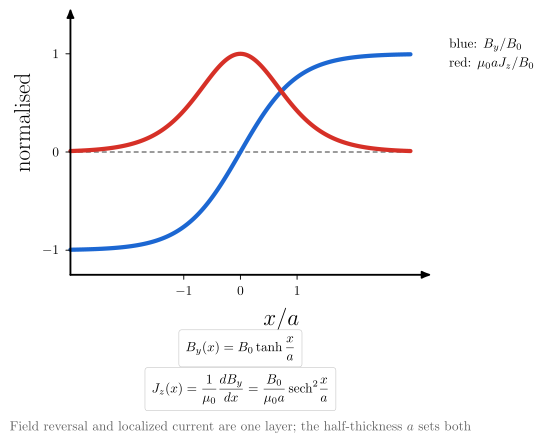
vaft.diagram.harris_sheet()$B_y(x)$ and $J_z(x)$ of the Harris sheet on one chart.
vaft.diagram.harris_sheet(*, labels=True)Show source vaft/diagram/_field_configurations.py, lines 259–293
def harris_sheet(*, labels: bool = True) -> Diagram:
    r"""$B_y(x)$ and $J_z(x)$ of the Harris sheet on one chart.

    ``harris_sheet_field`` normalised to $B_0$ and
    ``harris_sheet_current_density`` normalised to $B_0/(\mu_0a)$ over
    $|x| \le 3a$: the reversal of $B_y$ and the localized current are the same
    layer, $J_z = \mu_0^{-1}dB_y/dx$.
    """
    labels = _check_labels(labels)
    x = np.linspace(-3.0, 3.0, 301)
    b = harris_sheet_field(x * _A, _B0, _A) / _B0
    j = harris_sheet_current_density(x * _A, _B0, _A) / (_B0 / (MU0 * _A))
    chart = Chart(x_range=(-3.0, 3.0), y_range=(-1.25, 1.25))
    chart.curves.update({"B_y": np.stack([x, b], -1), "J_z": np.stack([x, j], -1),
                         "zero": np.array([[-3.0, 0.0], [3.0, 0.0]])})
    chart.parameters.update({"B0": _B0, "a": _A})
    scene = render_chart(chart, x_label="$x/a$", y_label="normalised",
                         curve_styles={"zero": "approx", "B_y": "component imag", "J_z": "component real"},
                         region_text={}, x_ticks=(-1.0, 0.0, 1.0), x_tick_text=("$-1$", "$0$", "$1$"),
                         y_ticks=(-1.0, 0.0, 1.0), y_tick_text=("$-1$", "$0$", "$1$"))
    items = list(scene.items)
    if labels:
        items += [
            Label((CHART_WIDTH + 0.9, CHART_HEIGHT - 0.1), "blue: $B_y/B_0$", "small label", anchor="north west",
                  role="legend"),
            Label((CHART_WIDTH + 0.9, CHART_HEIGHT - 0.6), "red: $\\mu_0aJ_z/B_0$", "small label",
                  anchor="north west", role="legend"),
            Label((CHART_WIDTH / 2, -1.45), f"$\\displaystyle {formula_equation(harris_sheet_field)}$",
                  "formula box", anchor="north", role="equations"),
            Label((CHART_WIDTH / 2, -2.45), f"$\\displaystyle {formula_equation(harris_sheet_current_density)}$",
                  "formula box", anchor="north", role="equations"),
            _note("Field reversal and localized current are one layer; the half-thickness $a$ sets both",
                  CHART_WIDTH / 2, -3.75),
        ]
    return Diagram("harris_sheet", Scene(tuple(items)), model=chart)
Formats .svg .tex .pdf the SVG above is committed; build the others locally
import vaft.diagram

d = vaft.diagram.harris_sheet()
d.tikz  # the TikZ document as text
d.save("harris_sheet.svg")  # rendered vector image, the canonical artifact; needs latex, dvisvgm
d.save("harris_sheet.tex")  # the complete TikZ document, the text source
d.save("harris_sheet.pdf")  # vector PDF; needs pdflatex
Formula functions referenced:
geometry.harris_sheet_current_density, geometry.harris_sheet_field
x_point
1 asset
source
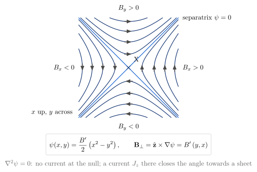
vaft.diagram.x_point()The current-free magnetic X-point of x_point_flux: four branches and two separatrices.
vaft.diagram.x_point(*, labels=True)Show source vaft/diagram/_field_configurations.py, lines 328–364
def x_point(*, labels: bool = True) -> Diagram:
    r"""The current-free magnetic X-point of ``x_point_flux``: four branches and two separatrices.

    Contours of $\psi = \tfrac12B'(x^2 - y^2)$ with $x$ up and $y$ across;
    arrows along $\mathbf B_\perp = B'(y, x)$. The separatrices $y = \pm x$
    ($\psi = 0$) meet at right angles at the null and divide the plane into
    four families: the upper and lower ($\psi > 0$) field lines have $B_y$ of
    opposite sign, as across a current sheet; the left and right ($\psi < 0$)
    ones $B_x$. Geometry only: no flow is implied (see
    ``magnetic_reconnection``).
    """
    labels = _check_labels(labels)
    L = 2.6
    levels = [s * v for v in (0.25, 0.9, 1.8, 2.9) for s in (1.0, -1.0)]
    items: List = []
    lines = _flux_lines(L, L, 1.0, levels)
    for line in lines:
        items.append(Polyline.of(line, "orbit electron", role="field_line"))
        items.append(_direction_arrow(line, 1.0, "field arrow", "field_direction"))
    for s in (1.0, -1.0):
        items.append(Polyline.of([(-L, -s * L), (L, s * L)], "separatrix", role="separatrix"))
    items.append(Marker((0.0, 0.0), "x", "xpoint", role="x_point"))
    if labels:
        items += [
            Label((0.15, 0.2), "X", "small label", anchor="south west", role="x_point"),
            Label((L + 0.1, L), "separatrix $\\psi = 0$", "small label", anchor="west", role="separatrix"),
            Label((0.0, L + 0.2), "$B_y > 0$", "small label", anchor="south", role="branch"),
            Label((0.0, -L - 0.2), "$B_y < 0$", "small label", anchor="north", role="branch"),
            Label((L + 0.1, 0.0), "$B_x > 0$", "small label", anchor="west", role="branch"),
            Label((-L - 0.1, 0.0), "$B_x < 0$", "small label", anchor="east", role="branch"),
            Label((-L - 0.2, -L), "$x$ up, $y$ across", "small label", anchor="south east", role="axes"),
            Label((0.0, -L - 0.85), f"$\\displaystyle {formula_equation(x_point_flux)}$", "formula box",
                  anchor="north", role="equations"),
            _note("$\\nabla^2\\psi = 0$: no current at the null; a current $J_z$ there closes the angle "
                  "towards a sheet", 0.0, -L - 2.1),
        ]
    return Diagram("x_point", Scene(tuple(items)), model={"levels": levels, "lines": lines})
Formats .svg .tex .pdf the SVG above is committed; build the others locally
import vaft.diagram

d = vaft.diagram.x_point()
d.tikz  # the TikZ document as text
d.save("x_point.svg")  # rendered vector image, the canonical artifact; needs latex, dvisvgm
d.save("x_point.tex")  # the complete TikZ document, the text source
d.save("x_point.pdf")  # vector PDF; needs pdflatex
Formula functions referenced:
geometry.x_point_flux
magnetic_reconnection
1 asset
source
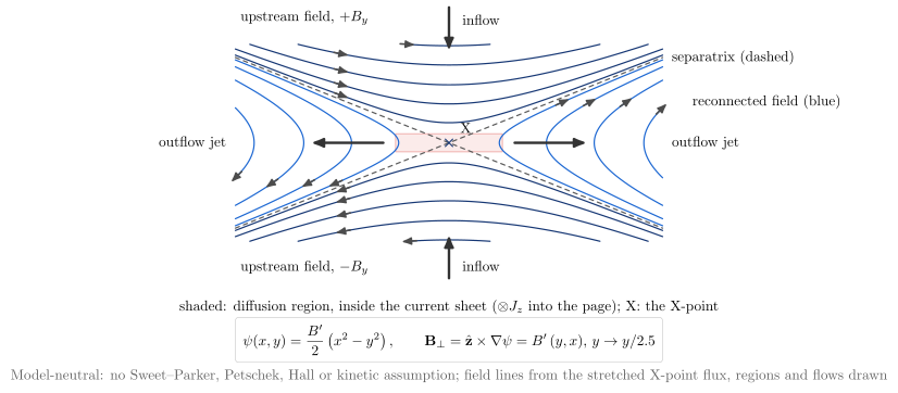
vaft.diagram.magnetic_reconnection()Model-neutral 2-D reconnection: inflow, outflow, diffusion region, upstream and reconnected field.
vaft.diagram.magnetic_reconnection(*, labels=True)Show source vaft/diagram/_field_configurations.py, lines 367–426
def magnetic_reconnection(*, labels: bool = True) -> Diagram:
    r"""Model-neutral 2-D reconnection: inflow, outflow, diffusion region, upstream and reconnected field.

    Field lines are contours of ``x_point_flux`` with $y$ stretched by 2.5,
    the X-point opened into a short current sheet; the diffusion region
    (shaded) and the flows are drawn, not solved. Upstream field lines
    ($\psi > 0$, dark) carry $\pm B_y$ in from above and below; reconnected
    field lines ($\psi < 0$, blue) leave to the sides with the outflow jets.
    No Sweet--Parker, Petschek, Hall or kinetic assumption is made; a guide
    field would be $\otimes$ along $z$ and leave this in-plane picture.
    """
    labels = _check_labels(labels)
    stretch, Ly, Lx = 2.5, 5.2, 2.4
    up = [0.12, 0.45, 1.0, 1.8, 2.8]
    down = [-v for v in (0.12, 0.45, 1.0, 1.8, 2.8)]
    items: List = []
    sheet = (1.3, 0.22)
    items.append(Polyline.of([(-sheet[0], -sheet[1]), (sheet[0], -sheet[1]), (sheet[0], sheet[1]),
                              (-sheet[0], sheet[1])], "layer", role="diffusion_region", closed=True))
    upstream = _flux_lines(Ly, Lx, stretch, up)
    reconnected = _flux_lines(Ly, Lx, stretch, down)
    for line in upstream:
        items.append(Polyline.of(line, "orbit electron", role="upstream_field"))
        items.append(_direction_arrow(line, stretch, "field arrow", "field_direction", (0, -2.6)))
    for line in reconnected:
        items.append(Polyline.of(line, "orbit ion", role="reconnected_field"))
        side = 1.0 if line[:, 0].mean() > 0 else -1.0
        items.append(_direction_arrow(line, stretch, "field arrow", "field_direction", (1, 1.0 * side)))
    for s in (1.0, -1.0):
        items.append(Polyline.of([(-Ly, -s * Ly / stretch), (Ly, s * Ly / stretch)], "approx",
                                 role="separatrix"))
    items.append(Marker((0.0, 0.0), "x", "xpoint", role="x_point"))
    items += [Arrow((0.0, Lx + 0.9), (0.0, Lx - 0.2), "exb", role="inflow"),
              Arrow((0.0, -Lx - 0.9), (0.0, -Lx + 0.2), "exb", role="inflow"),
              Arrow((1.6, 0.0), (3.4, 0.0), "exb", role="outflow"),
              Arrow((-1.6, 0.0), (-3.4, 0.0), "exb", role="outflow")]
    if labels:
        items += [
            Label((0.2, Lx + 0.6), "inflow", "small label", anchor="west", role="inflow"),
            Label((0.2, -Lx - 0.6), "inflow", "small label", anchor="west", role="inflow"),
            Label((Ly + 0.1, 0.0), "outflow jet", "small label", anchor="west", role="outflow"),
            Label((-Ly - 0.1, 0.0), "outflow jet", "small label", anchor="east", role="outflow"),
            Label((-Ly, Lx + 0.35), "upstream field, $+B_y$", "small label", anchor="south west",
                  role="upstream_field"),
            Label((-Ly, -Lx - 0.35), "upstream field, $-B_y$", "small label", anchor="north west",
                  role="upstream_field"),
            Label((0.15, 0.12), "X", "small label", anchor="south west", role="x_point"),
            Label((Ly + 0.6, 1.0), "reconnected field (blue)", "small label", anchor="west",
                  role="reconnected_field"),
            Label((Ly + 0.1, Ly / stretch), "separatrix (dashed)", "small label", anchor="west", role="separatrix"),
            Label((0.0, -Lx - 1.3), "shaded: diffusion region, inside the current sheet ($\\otimes J_z$ into "
                  "the page); X: the X-point",
                  "small label", anchor="north", role="diffusion_region"),
            Label((0.0, -Lx - 1.85), f"$\\displaystyle {formula_equation(x_point_flux)}$, $y \\to y/{stretch:g}$",
                  "formula box", anchor="north", role="equations"),
            _note("Model-neutral: no Sweet--Parker, Petschek, Hall or kinetic assumption; field lines from the "
                  "stretched X-point flux, regions and flows drawn", 0.0, -Lx - 3.0),
        ]
    return Diagram("magnetic_reconnection", Scene(tuple(items)),
                   model={"stretch": stretch, "upstream": upstream, "reconnected": reconnected})
Formats .svg .tex .pdf the SVG above is committed; build the others locally
import vaft.diagram

d = vaft.diagram.magnetic_reconnection()
d.tikz  # the TikZ document as text
d.save("magnetic_reconnection.svg")  # rendered vector image, the canonical artifact; needs latex, dvisvgm
d.save("magnetic_reconnection.tex")  # the complete TikZ document, the text source
d.save("magnetic_reconnection.pdf")  # vector PDF; needs pdflatex
Formula functions referenced:
geometry.x_point_flux
island_formation
1 asset
source
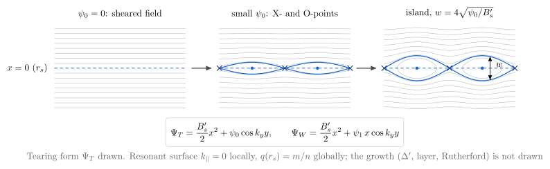
vaft.diagram.island_formation()From a sheared field to a magnetic island: slab_perturbed_flux with growing tearing amplitude.
vaft.diagram.island_formation(*, labels=True)Show source vaft/diagram/_field_configurations.py, lines 437–504
def island_formation(*, labels: bool = True) -> Diagram:
    r"""From a sheared field to a magnetic island: ``slab_perturbed_flux`` with growing tearing amplitude.

    Three panels of constant-$\Psi$ contours over two wavelengths:
    $\psi_0 = 0$, the straight sheared field lines with the resonant surface
    $x = 0$ ($k_\parallel = 0$); a small $\psi_0$, where the field lines
    reconnect at X-points and close around O-points; a larger $\psi_0$, the
    island of full width $w = 4\sqrt{\psi_0/B'}$ bounded by its separatrix.
    The dynamics that grow $\psi_0$ -- $\Delta'$, the layer, Rutherford -- are
    ``delta_prime``, ``slab_parity`` and ``tearing_layer_matching``.
    """
    labels = _check_labels(labels)
    k_y, shear = 1.0, 1.0
    wavelength = 2.0 * math.pi / k_y
    W, Hh, gap = 5.0, 1.6, 1.3  # panel width, half-height [cm], gap
    # 301 samples: grid nodes land at multiples of W/300 cm, never on a 4-decimal rounding tie (321 would put
    # them at k/64 cm, where last-bit differences between platforms flip the printed coordinate)
    ys = np.linspace(0.0, 2.0 * wavelength, 301)
    xs = np.linspace(-1.0, 1.0, 157)  # no contour level falls on a grid row (161 put d = 0.95 on one)
    Y, X = np.meshgrid(ys, xs)
    items: List = []
    widths, separatrices = [], []
    for i, amp in enumerate(_STAGES):
        x0 = i * (W + gap)

        def cm(pts, x0=x0):
            pts = np.asarray(pts, dtype=float)
            return np.stack([x0 + pts[..., 0] / (2.0 * wavelength) * W, pts[..., 1] * Hh], -1)

        Z = slab_perturbed_flux(X, Y, shear, amp, k_y)
        levels = [0.5 * shear * d * d for d in np.linspace(0.12, 0.95, 8)]
        for line in _contours(Z, xs, ys, levels):
            items.append(Polyline.of(cm(line), "surface", role=f"flux_surface:{i}"))
        items.append(Polyline.of(cm([[0.0, 0.0], [2.0 * wavelength, 0.0]]), "rational", role=f"resonant_surface:{i}"))
        width = 4.0 * math.sqrt(amp / shear)
        widths.append(width)
        if amp > 0.0:
            # a hair inside the saddle value: exactly at it the X-points sit on grid nodes and a last-bit
            # difference in cos(k_y y) decides how contourpy joins the lines, platform by platform
            lines = _contours(Z, xs, ys, [amp * (1.0 - 1e-6)])
            separatrices.append(lines)
            for line in lines:
                items.append(Polyline.of(cm(line), "separatrix", role=f"separatrix:{i}"))
            for yy in (0.0, wavelength, 2.0 * wavelength):
                items.append(Marker(tuple(cm((yy, 0.0))), "x", "xpoint", role=f"x_point:{i}"))
            for yy in (0.5 * wavelength, 1.5 * wavelength):
                items.append(Marker(tuple(cm((yy, 0.0))), "o", "opoint", role=f"o_point:{i}"))
        if i:
            items.append(Arrow((x0 - gap + 0.25, 0.0), (x0 - 0.25, 0.0), "connector", role="stage"))
        if labels:
            title = ("$\\psi_0 = 0$: sheared field", "small $\\psi_0$: X- and O-points",
                     "island, $w = 4\\sqrt{\\psi_0/B_s'}$")[i]
            items.append(Label((x0 + 0.5 * W, Hh + 0.2), title, "small label", anchor="south", role="title"))
        if labels and i == 2:
            yo = cm((1.5 * wavelength, 0.0))
            items += [Arrow((float(yo[0]) + 0.3, -0.5 * width * Hh), (float(yo[0]) + 0.3, 0.5 * width * Hh),
                            "width arrow", role="width", both=True),
                      Label((float(yo[0]) + 0.4, 0.12), "$w$", "small label", anchor="west", role="width")]
    if labels:
        items += [
            Label((-0.15, 0.0), "$x = 0$ ($r_s$)", "small label", anchor="east", role="resonant_surface"),
            Label((1.5 * W + gap, -Hh - 0.3), f"$\\displaystyle {formula_equation(slab_perturbed_flux)}$",
                  "formula box", anchor="north", role="equations"),
            _note("Tearing form $\\Psi_T$ drawn. Resonant surface $k_\\parallel = 0$ locally, $q(r_s) = m/n$ "
                  "globally; the growth ($\\Delta'$, layer, Rutherford) is not drawn", 1.5 * W + gap, -Hh - 1.5),
        ]
    return Diagram("island_formation", Scene(tuple(items)), model={"amplitudes": _STAGES, "widths": widths,
                                                                 "separatrices": separatrices})
Formats .svg .tex .pdf the SVG above is committed; build the others locally
import vaft.diagram

d = vaft.diagram.island_formation()
d.tikz  # the TikZ document as text
d.save("island_formation.svg")  # rendered vector image, the canonical artifact; needs latex, dvisvgm
d.save("island_formation.tex")  # the complete TikZ document, the text source
d.save("island_formation.pdf")  # vector PDF; needs pdflatex
Formula functions referenced:
stability.slab_perturbed_flux
Linear ideal-MHD waves in a uniform plasma: polarization and the branch family
Module vaft.diagram._mhd_waves
shear_alfven_wave
1 asset
source
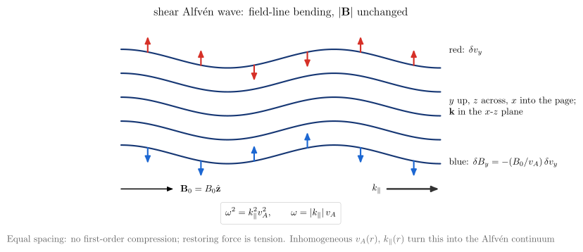
vaft.diagram.shear_alfven_wave()Shear Alfven polarization: field-line bending without compression.
vaft.diagram.shear_alfven_wave(*, labels=True)Show source vaft/diagram/_mhd_waves.py, lines 47–108
def shear_alfven_wave(*, labels: bool = True) -> Diagram:
    r"""Shear Alfven polarization: field-line bending without compression.

    $\mathbf B_0 = B_0\hat{\mathbf z}$ across the page, the displacement
    $\xi_y = \xi_0\cos(k_\parallel z - \omega t)$ up, at $t = 0$, over one and
    a half wavelengths. Every field line is displaced alike, so the spacing
    -- $|\mathbf B|$ -- is unchanged to first order and the restoring force is
    tension alone. Red: $\delta v_y = \partial_t\xi_y$; blue:
    $\delta B_y = B_0\partial_z\xi_y = -(B_0/v_A)\,\delta v_y$ for the wave
    travelling along $+\mathbf B_0$, with $\omega$ from
    ``shear_alfven_frequency``. Both are along $\hat{\mathbf y}$, normal to the
    $\mathbf k$-$\mathbf B_0$ plane; $\omega$ does not depend on $k_\perp$.
    """
    labels = _check_labels(labels)
    L, n_lines, dy = 12.0, 5, 0.9  # page width [cm], field lines, spacing [cm]
    wavelength = L / 1.5
    k = 2.0 * math.pi / wavelength
    omega = float(shear_alfven_frequency(k, _VA))
    xi0 = 0.35
    z = np.linspace(0.0, L, 361)
    items: List = []
    lines = []
    for j in range(n_lines):
        y0 = (j - (n_lines - 1) / 2) * dy
        y = y0 + xi0 * np.cos(k * z)
        lines.append(np.stack([z, y], -1))
        items.append(Polyline.of(lines[-1], "field line", role="field_line"))
    zs = wavelength / 8 + np.arange(8) * wavelength / 4  # off the nodes of sin(kz)
    zs = zs[zs < L - 0.2]
    scale_v, scale_b = 0.9 / (omega * xi0), 0.9 / (_B0 * k * xi0)
    y_top = (n_lines - 1) / 2 * dy
    samples = []
    for zz in zs:
        dv = omega * xi0 * math.sin(k * zz)  # d/dt of xi0 cos(kz - wt) at t = 0
        dB = -_B0 * k * xi0 * math.sin(k * zz)
        base_v = y_top + xi0 * math.cos(k * zz)
        base_b = -y_top + xi0 * math.cos(k * zz)
        samples.append((zz, dv, dB))
        if abs(dv) > 1e-9:
            items.append(Arrow((zz, base_v), (zz, base_v + scale_v * dv), "drift", role="delta_v"))
            items.append(Arrow((zz, base_b), (zz, base_b + scale_b * dB), "drift ion", role="delta_B"))
    base = -(n_lines + 1) / 2 * dy - 0.4
    items += [Arrow((0.0, base), (2.0, base), "vector", role="B0"),
              Arrow((L - 2.0, base), (L, base), "exb", role="k")]
    if labels:
        items += [
            Label((2.1, base), "$\\mathbf{B}_0 = B_0\\hat{\\mathbf{z}}$", "small label", anchor="west", role="B0"),
            Label((L - 2.1, base), "$k_\\parallel$", "small label", anchor="east", role="k"),
            Label((L + 0.2, y_top + 0.3), "red: $\\delta v_y$", "small label", anchor="west", role="legend"),
            Label((L + 0.2, -y_top - 0.3), "blue: $\\delta B_y = -(B_0/v_A)\\,\\delta v_y$", "small label",
                  anchor="west", role="legend"),
            Label((L + 0.2, 0.0), "$y$ up, $z$ across, $x$ into the page;\\\\ $\\mathbf{k}$ in the $x$-$z$ plane",
                  "small label,align=left", anchor="west", role="axes"),
            Label((0.5 * L, y_top + 1.4), "shear Alfv\\'en wave: field-line bending, $|\\mathbf{B}|$ unchanged",
                  "label", anchor="south", role="title"),
            Label((0.5 * L, base - 0.5), f"$\\displaystyle {formula_equation(shear_alfven_frequency)}$",
                  "formula box", anchor="north", role="equations"),
            _note("Equal spacing: no first-order compression; restoring force is tension. Inhomogeneous "
                  "$v_A(r)$, $k_\\parallel(r)$ turn this into the Alfv\\'en continuum", 0.5 * L, base - 1.6),
        ]
    return Diagram("shear_alfven_wave", Scene(tuple(items)),
                   model={"k": k, "omega": omega, "xi0": xi0, "lines": lines, "samples": samples})
Formats .svg .tex .pdf the SVG above is committed; build the others locally
import vaft.diagram

d = vaft.diagram.shear_alfven_wave()
d.tikz  # the TikZ document as text
d.save("shear_alfven_wave.svg")  # rendered vector image, the canonical artifact; needs latex, dvisvgm
d.save("shear_alfven_wave.tex")  # the complete TikZ document, the text source
d.save("shear_alfven_wave.pdf")  # vector PDF; needs pdflatex
Formula functions referenced:
stability.shear_alfven_frequency
fast_magnetosonic_wave
1 asset
source
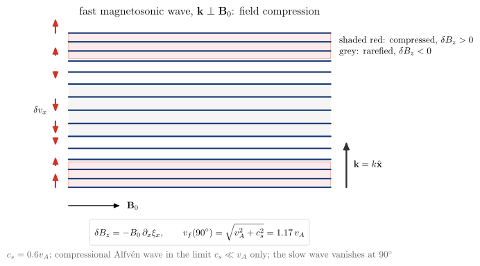
vaft.diagram.fast_magnetosonic_wave()Fast magnetosonic polarization at $\mathbf k \perp \mathbf B_0$: compression and rarefaction.
vaft.diagram.fast_magnetosonic_wave(*, labels=True)Show source vaft/diagram/_mhd_waves.py, lines 111–170
def fast_magnetosonic_wave(*, labels: bool = True) -> Diagram:
    r"""Fast magnetosonic polarization at $\mathbf k \perp \mathbf B_0$: compression and rarefaction.

    $\mathbf B_0$ across the page, $\mathbf k = k\hat{\mathbf x}$ up, the
    displacement $\xi_x = \xi_0\sin(kx - \omega t)$ at $t = 0$ along
    $\mathbf k$: field lines bunch where $\partial_x\xi_x < 0$ and spread
    where it is positive, $\delta B_z = -B_0\partial_x\xi_x$. Magnetic and
    thermal pressure rise together, the restoring force of the fast wave,
    whose speed here is ``magnetosonic_phase_speeds`` at $\theta = 90^\circ$,
    $\sqrt{v_A^2 + c_s^2}$; for $c_s \ll v_A$ it is the compressional Alfven
    wave $\omega \simeq kv_A$. At other angles the fast and slow branches mix
    compression with bending (``mhd_wave_family``).
    """
    labels = _check_labels(labels)
    L, n_lines, dx = 10.0, 15, 0.42  # page width [cm], field lines, unperturbed spacing [cm]
    height = (n_lines - 1) * dx
    k = 2.0 * math.pi / height
    xi0 = 0.2
    fast, slow = magnetosonic_phase_speeds(0.5 * math.pi, _VA, _CS)
    x0s = (np.arange(n_lines) - (n_lines - 1) / 2) * dx
    xs = x0s + xi0 * np.sin(k * x0s)
    items: List = []
    # compressed (dxi/dx < 0) and rarefied bands, from delta B_z = -B0 dxi/dx
    grid = np.linspace(x0s[0], x0s[-1], 721)
    dBz = -_B0 * k * xi0 * np.cos(k * grid)
    for sign, style, role in ((1.0, "layer", "compressed"), (-1.0, "concept band", "rarefied")):
        inside = sign * dBz > 0.5 * _B0 * k * xi0
        edges = np.flatnonzero(np.diff(inside.astype(int)))
        runs = np.split(np.arange(len(grid)), edges + 1)
        for run in runs:
            if inside[run[0]]:
                a, b = grid[run[0]], grid[run[-1]]
                items.append(Polyline.of([(0.0, a), (L, a), (L, b), (0.0, b)], style, role=role, closed=True))
    for x in xs:
        items.append(Polyline.of([(0.0, x), (L, x)], "field line", role="field_line"))
    for x in x0s[::2]:
        v = -xi0 * math.cos(k * x)  # d/dt of xi0 sin(kx - wt) at t = 0, per unit omega
        if abs(v) > 1e-3:
            items.append(Arrow((-0.5, x), (-0.5, x + 3.0 * v), "drift", role="delta_v"))
    items += [Arrow((L + 0.6, x0s[0]), (L + 0.6, x0s[0] + 1.8), "exb", role="k"),
              Arrow((0.0, x0s[0] - 0.7), (2.0, x0s[0] - 0.7), "vector", role="B0")]
    if labels:
        items += [
            Label((L + 0.75, x0s[0] + 0.9), "$\\mathbf{k} = k\\hat{\\mathbf{x}}$", "small label", anchor="west",
                  role="k"),
            Label((2.1, x0s[0] - 0.7), "$\\mathbf{B}_0$", "small label", anchor="west", role="B0"),
            Label((-0.7, 0.0), "$\\delta v_x$", "small label", anchor="east", role="delta_v"),
            Label((L + 0.2, x0s[-1]), "shaded red: compressed, $\\delta B_z > 0$\\\\ grey: rarefied, "
                  "$\\delta B_z < 0$", "small label,align=left", anchor="north west", role="legend"),
            Label((0.5 * L, x0s[-1] + 0.5), "fast magnetosonic wave, $\\mathbf{k} \\perp \\mathbf{B}_0$: "
                  "field compression", "label", anchor="south", role="title"),
            Label((0.5 * L, x0s[0] - 1.2),
                  "$\\displaystyle \\delta B_z = -B_0\\,\\partial_x\\xi_x,\\qquad v_f(90^\\circ) = "
                  f"\\sqrt{{v_A^2 + c_s^2}} = {float(fast):.2f}\\,v_A$", "formula box", anchor="north",
                  role="equations"),
            _note(f"$c_s = {_CS:g}v_A$; compressional Alfv\\'en wave in the limit $c_s \\ll v_A$ only; "
                  "the slow wave vanishes at $90^\\circ$", 0.5 * L, x0s[0] - 2.3),
        ]
    return Diagram("fast_magnetosonic_wave", Scene(tuple(items)),
                   model={"k": k, "xi0": xi0, "positions": xs, "v_fast": float(fast), "v_slow": float(slow)})
Formats .svg .tex .pdf the SVG above is committed; build the others locally
import vaft.diagram

d = vaft.diagram.fast_magnetosonic_wave()
d.tikz  # the TikZ document as text
d.save("fast_magnetosonic_wave.svg")  # rendered vector image, the canonical artifact; needs latex, dvisvgm
d.save("fast_magnetosonic_wave.tex")  # the complete TikZ document, the text source
d.save("fast_magnetosonic_wave.pdf")  # vector PDF; needs pdflatex
Formula functions referenced:
stability.magnetosonic_phase_speeds
mhd_wave_family
1 asset
source
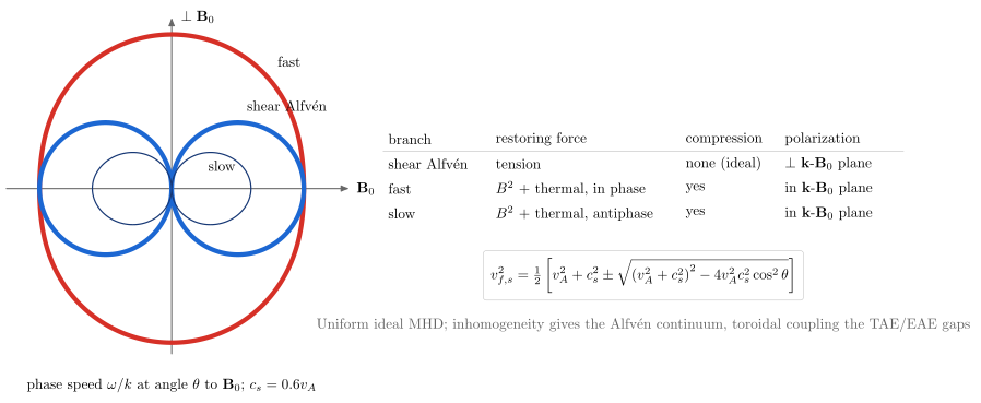
vaft.diagram.mhd_wave_family()The Friedrichs diagram: phase speed against the angle to $\mathbf B_0$, three branches.
vaft.diagram.mhd_wave_family(*, labels=True)Show source vaft/diagram/_mhd_waves.py, lines 173–225
def mhd_wave_family(*, labels: bool = True) -> Diagram:
    r"""The Friedrichs diagram: phase speed against the angle to $\mathbf B_0$, three branches.

    Polar curves of the phase speed at angle $\theta$ between $\mathbf k$ and
    $\mathbf B_0$ (horizontal) for $c_s = 0.6v_A$: fast and slow from
    ``magnetosonic_phase_speeds``, shear Alfven $v_A|\cos\theta|$ from
    ``shear_alfven_frequency``$/k$ -- two circles through the origin. At every
    angle $v_s \le v_A|\cos\theta| \le v_f$. Beside it, what restores each
    branch, whether it compresses, and its polarization.
    """
    labels = _check_labels(labels)
    theta = np.linspace(0.0, 2.0 * math.pi, 721)
    fast, slow = magnetosonic_phase_speeds(theta, _VA, _CS)
    alfven = shear_alfven_frequency(np.cos(theta), _VA)  # omega/k with k = 1
    S = 3.2  # cm per v_A
    curves = {"fast": fast, "alfven": alfven, "slow": slow}
    styles = {"fast": "component real", "alfven": "component imag", "slow": "orbit electron"}
    items: List = [Arrow((-1.25 * S, 0.0), (1.35 * S, 0.0), "frame axis arrow", role="axes"),
                   Arrow((0.0, -1.25 * S), (0.0, 1.3 * S), "frame axis arrow", role="axes")]
    for name, v in curves.items():
        items.append(Polyline.of(np.stack([S * v * np.cos(theta), S * v * np.sin(theta)], -1), styles[name],
                                 role=name, closed=True))
    if labels:
        t = math.radians(50.0)
        f50, s50 = magnetosonic_phase_speeds(t, _VA, _CS)
        items += [
            Label((1.36 * S, 0.0), "$\\mathbf{B}_0$", "small label", anchor="west", role="axes"),
            Label((0.1, 1.3 * S), "$\\perp\\mathbf{B}_0$", "small label", anchor="west", role="axes"),
            Label((S * float(f50) * math.cos(t) + 0.15, S * float(f50) * math.sin(t) + 0.1), "fast",
                  "small label", anchor="south west", role="fast"),
            Label((S * 0.5 * _VA + 0.1, S * 0.55 * _VA), "shear Alfv\\'en", "small label", anchor="south west",
                  role="alfven"),
            Label((S * float(s50) * math.cos(t) + 0.05, S * float(s50) * math.sin(t) - 0.05), "slow",
                  "small label", anchor="north west", role="slow"),
            Label((0.0, -1.3 * S - 0.3), f"phase speed $\\omega/k$ at angle $\\theta$ to $\\mathbf{{B}}_0$; "
                  f"$c_s = {_CS:g}v_A$", "small label", anchor="north", role="axes"),
        ]
        rows = [("branch", "restoring force", "compression", "polarization"),
                ("shear Alfv\\'en", "tension", "none (ideal)", "$\\perp$ $\\mathbf{k}$-$\\mathbf{B}_0$ plane"),
                ("fast", "$B^2$ + thermal, in phase", "yes", "in $\\mathbf{k}$-$\\mathbf{B}_0$ plane"),
                ("slow", "$B^2$ + thermal, antiphase", "yes", "in $\\mathbf{k}$-$\\mathbf{B}_0$ plane")]
        x0, cols = 1.6 * S, (0.0, 2.6, 7.2, 9.6)
        for j, row in enumerate(rows):
            for c, text in zip(cols, row):
                items.append(Label((x0 + c, 1.2 - 0.6 * j), text, "small label", anchor="west",
                                   role="table:head" if j == 0 else "table"))
        items.append(Polyline.of([(x0, 0.9), (x0 + 12.6, 0.9)], "surface", role="table"))
        items.append(Label((x0 + 6.3, -1.5), f"$\\displaystyle {formula_equation(magnetosonic_phase_speeds)}$",
                           "formula box", anchor="north", role="equations"))
        items.append(_note("Uniform ideal MHD; inhomogeneity gives the Alfv\\'en continuum, toroidal coupling "
                           "the TAE/EAE gaps", x0 + 6.3, -3.0))
    return Diagram("mhd_wave_family", Scene(tuple(items)),
                   model={"theta": theta, "fast": fast, "alfven": alfven, "slow": slow, "c_s": _CS, "v_A": _VA})
Formats .svg .tex .pdf the SVG above is committed; build the others locally
import vaft.diagram
d = vaft.diagram.mhd_wave_family()
d.tikz # the TikZ document as text
d.save("mhd_wave_family.svg") # rendered vector image, the canonical artifact; needs latex, dvisvgm
d.save("mhd_wave_family.tex") # the complete TikZ document, the text source
d.save("mhd_wave_family.pdf") # vector PDF; needs pdflatexFormula functions referenced:
stability.magnetosonic_phase_speeds, stability.shear_alfven_frequency
Plasma-wall interaction concepts: processes, reflection, sputtering, recycling, energy partition, and the
Module vaft.diagram._pwi
plasma_wall_interaction_processes
1 asset
source
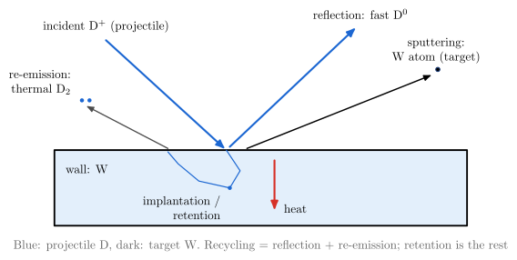
vaft.diagram.plasma_wall_interaction_processes()One ion impact and its outcomes, the projectile and target species kept apart.
vaft.diagram.plasma_wall_interaction_processes(projectile='D', target='W', *, labels=True)Show source vaft/diagram/_pwi.py, lines 105–157
def plasma_wall_interaction_processes(projectile="D", target="W", *, labels: bool = True) -> Diagram:
r"""One ion impact and its outcomes, the projectile and target species kept apart.
An incident ion (projectile, blue) strikes the wall (target material,
grey): it may be reflected at once as a fast atom; or implanted, where
it stays (retention) or later diffuses back out, recombines and leaves as
a thermal molecule (re-emission); it may knock a target atom out
(sputtering, dark); and the energy it does not carry away is deposited as
heat. Reflection plus re-emission is recycling. Semantic: no
coefficients.
"""
labels = _check_labels(labels)
p, t = _species(projectile), _species(target)
items: List = _wall(0.0, 12.0)
hit = (5.0, 0.0)
items.append(Arrow((1.5, 3.2), hit, "drift ion", role="incident"))
outcomes = {
"reflection": ((8.8, 3.6), True),
"sputtering": ((11.0, 2.2), False),
"re-emission": ((0.9, 1.3), True),
}
items.append(Arrow((hit[0] + 0.1, 0.1), outcomes["reflection"][0], "drift ion", role="outcome:reflection"))
items.append(Arrow((hit[0] + 0.6, 0.05), outcomes["sputtering"][0], "vector", role="outcome:sputtering"))
items.append(_atom(outcomes["sputtering"][0][0] + 0.15, outcomes["sputtering"][0][1] + 0.15, False,
"sputtered_atom"))
# implantation: the ion comes to rest inside; some diffuses back and leaves as a molecule
items.append(Polyline.of([hit, (5.4, -0.6), (5.1, -1.1)], "orbit ion", role="implantation"))
items.append(_atom(5.1, -1.1, True, "implanted"))
items.append(Polyline.of([(5.1, -1.1), (4.2, -0.9), (3.6, -0.4), (3.3, -0.05)], "orbit ion",
role="diffusion_back"))
items.append(Arrow((3.3, 0.05), outcomes["re-emission"][0], "connector", role="outcome:re-emission"))
for dx in (0.0, 0.22):
items.append(_atom(outcomes["re-emission"][0][0] - 0.1 + dx, outcomes["re-emission"][0][1] + 0.15, True,
"molecule"))
items.append(Arrow((6.4, -0.3), (6.4, -1.8), "drift", role="heat"))
if labels:
items += [
Label((1.5, 3.3), f"incident {p}$^+$ (projectile)", "small label", anchor="south", role="incident"),
Label((8.9, 3.7), f"reflection: fast {p}$^0$", "small label", anchor="south", role="reflection"),
Label((11.1, 2.4), f"sputtering:\\\\ {t} atom (target)", "small label,align=center", anchor="south",
role="sputtering"),
Label((0.6, 1.5), f"re-emission:\\\\ thermal {p}$_2$", "small label,align=right", anchor="south east",
role="re-emission"),
Label((4.95, -1.2), "implantation /\\\\ retention", "small label,align=right", anchor="north east",
role="retention"),
Label((6.55, -1.7), "heat", "small label", anchor="west", role="heat"),
Label((0.2, -0.3), f"wall: {t}", "small label", anchor="north west", role="wall"),
_note(f"Blue: projectile {p}, dark: target {t}. Recycling = reflection + re-emission; retention is "
"the rest", 6.0, -2.5),
]
return Diagram("plasma_wall_interaction_processes", Scene(tuple(items)),
model={"projectile": p, "target": t, "outcomes": ("reflection", "implantation", "re-emission",
"sputtering", "heat"), "imas": IMAS_WALL_PATHS})Formats .svg .tex .pdf the SVG above is committed; build the others locally
import vaft.diagram
d = vaft.diagram.plasma_wall_interaction_processes()
d.tikz # the TikZ document as text
d.save("plasma_wall_interaction_processes.svg") # rendered vector image, the canonical artifact; needs latex, dvisvgm
d.save("plasma_wall_interaction_processes.tex") # the complete TikZ document, the text source
d.save("plasma_wall_interaction_processes.pdf") # vector PDF; needs pdflatexplasma_wall_interaction_reflection
1 asset
source
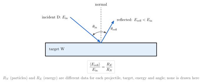
vaft.diagram.plasma_wall_interaction_reflection()Particle reflection: incident and reflected energy and angle are separate quantities.
vaft.diagram.plasma_wall_interaction_reflection(projectile='D', target='W', *, labels=True)Show source vaft/diagram/_pwi.py, lines 160–202
def plasma_wall_interaction_reflection(projectile="D", target="W", *, labels: bool = True) -> Diagram:
r"""Particle reflection: incident and reflected energy and angle are separate quantities.
An incident particle $(E_\mathrm{in}, \theta_\mathrm{in})$ and a
reflected one $(E_\mathrm{refl}, \theta_\mathrm{refl})$, angles from the
surface normal; the reflected particle leaves with less energy and at a
different angle, both distributed. $R_N$ counts reflected particles, $R_E$
reflected energy; their ratio is the mean reflected-energy fraction
(``mean_reflected_energy_fraction``). Both coefficients are data, not
drawn.
"""
labels = _check_labels(labels)
p, t = _species(projectile), _species(target)
items: List = _wall(0.0, 10.0, 1.2)
hit = (5.0, 0.0)
th_in, th_out = math.radians(50.0), math.radians(30.0)
L_in, L_out = 3.6, 2.4
start = (hit[0] - L_in * math.sin(th_in), L_in * math.cos(th_in))
end = (hit[0] + L_out * math.sin(th_out), L_out * math.cos(th_out))
items += [Polyline.of([hit, (hit[0], 3.2)], "approx", role="normal"),
Arrow(start, hit, "drift ion", role="incident"),
Arrow(hit, end, "drift ion", role="reflected")]
for th, sign, role in ((th_in, -1, "angle:in"), (th_out, 1, "angle:out")):
a = np.linspace(0.0, th, 30)
items.append(Polyline.of(np.stack([hit[0] + sign * 1.0 * np.sin(a), 1.0 * np.cos(a)], -1), "angle arc",
role=role))
if labels:
items += [
Label((start[0] - 0.1, start[1]), f"incident {p}: $E_\\mathrm{{in}}$", "small label", anchor="east",
role="incident"),
Label((end[0] + 0.1, end[1]), "reflected: $E_\\mathrm{refl} < E_\\mathrm{in}$", "small label",
anchor="west", role="reflected"),
Label((hit[0] - 0.55, 1.2), "$\\theta_\\mathrm{in}$", "small label", anchor="south", role="angle:in"),
Label((hit[0] + 0.75, 1.0), "$\\theta_\\mathrm{refl}$", "small label", anchor="south west", role="angle:out"),
Label((hit[0], 3.25), "normal", "small label", anchor="south", role="normal"),
Label((0.2, -0.3), f"target {t}", "small label", anchor="north west", role="wall"),
Label((5.0, -1.6), f"$\\displaystyle {formula_equation(mean_reflected_energy_fraction)}$", "formula box",
anchor="north", role="equations"),
_note("$R_N$ (particles) and $R_E$ (energy) are different data for each projectile, target, "
"energy and angle; none is drawn here", 5.0, -2.9),
]
return Diagram("plasma_wall_interaction_reflection", Scene(tuple(items)),
model={"projectile": p, "target": t, "theta_in": th_in, "theta_refl": th_out})Formats .svg .tex .pdf the SVG above is committed; build the others locally
import vaft.diagram
d = vaft.diagram.plasma_wall_interaction_reflection()
d.tikz # the TikZ document as text
d.save("plasma_wall_interaction_reflection.svg") # rendered vector image, the canonical artifact; needs latex, dvisvgm
d.save("plasma_wall_interaction_reflection.tex") # the complete TikZ document, the text source
d.save("plasma_wall_interaction_reflection.pdf") # vector PDF; needs pdflatexFormula functions referenced:
pwi.mean_reflected_energy_fraction
plasma_wall_interaction_sputtering
1 asset
source
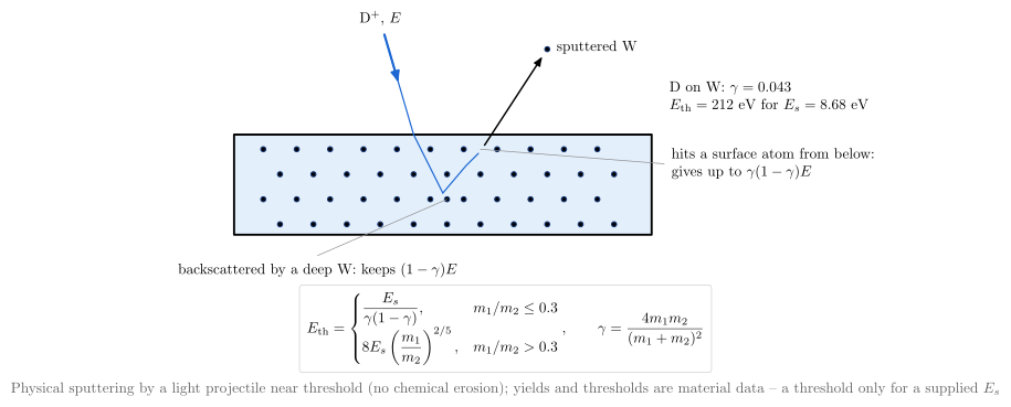
vaft.diagram.plasma_wall_interaction_sputtering(surface_binding_energy=8.68)Physical sputtering by a light projectile: backscatter from below ejects a surface atom.
vaft.diagram.plasma_wall_interaction_sputtering(projectile='D', target='W', surface_binding_energy=None, *, labels=True)Show source vaft/diagram/_pwi.py, lines 205–261
def plasma_wall_interaction_sputtering(projectile="D", target="W", surface_binding_energy: Optional[float] = None, *,
labels: bool = True) -> Diagram:
r"""Physical sputtering by a light projectile: backscatter from below ejects a surface atom.
For a light projectile (D on W) the route near threshold is: the
projectile penetrates, is backscattered by a deeper target atom keeping
$(1 - \gamma)E$, and on its way out strikes a surface atom from below,
giving it up to $\gamma(1 - \gamma)E$; if that exceeds the surface
binding energy the atom leaves. Hence Bohdansky's threshold
$E_s/\gamma(1 - \gamma)$, with $\gamma$ from
``binary_collision_energy_transfer_factor`` for the pair; the threshold is
drawn only if ``surface_binding_energy`` is given
(``sputtering_threshold_bohdansky``). No yield is drawn.
"""
labels = _check_labels(labels)
p, t = _species(projectile), _species(target)
if p not in MASS_U or t not in MASS_U:
raise ValueError(f"no mass tabulated here for {p if p not in MASS_U else t}")
gamma = float(binary_collision_energy_transfer_factor(MASS_U[p], MASS_U[t]))
E_th = None
if surface_binding_energy is not None:
E_th = float(sputtering_threshold_bohdansky(surface_binding_energy, MASS_U[p], MASS_U[t]))
items: List = _wall(0.0, 10.0, 2.4)
lattice = [(0.7 + 0.8 * i + (0.4 if j % 2 else 0.0), -0.35 - 0.6 * j) for j in range(4) for i in range(11)]
deep = (5.1, -1.55) # the target atom that backscatters the projectile
surface_atom = (5.9, -0.35) # the surface atom it strikes from below on the way out
for k, (x, y) in enumerate(lattice):
items.append(_atom(x, y, False, f"lattice:{k}"))
path_in = [(3.6, 2.4), (4.3, 0.0), (5.0, -1.4)]
path_out = [(5.0, -1.4), (5.55, -0.75), (5.85, -0.45)]
items += [Arrow(path_in[0], (3.95, 1.2), "drift ion", role="incident"),
Polyline.of(path_in, "orbit ion", role="projectile_in"),
Polyline.of(path_out, "orbit ion", role="projectile_backscattered"),
_atom(*deep, False, "backscatterer"),
Arrow((6.0, -0.25), (7.4, 1.9), "vector", role="sputtered"),
_atom(7.5, 2.05, False, "sputtered_atom")]
if labels:
items += [
Label((3.5, 2.5), f"{p}$^+$, $E$", "small label", anchor="south", role="incident"),
Label((7.6, 2.1), f"sputtered {t}", "small label", anchor="west", role="sputtered"),
Polyline.of([deep, (2.0, -2.9)], "leader line", role="backscatter"),
Label((2.0, -2.95), f"backscattered by a deep {t}: keeps $(1-\\gamma)E$", "small label", anchor="north",
role="backscatter"),
Polyline.of([surface_atom, (10.3, -0.7)], "leader line", role="transfer"),
Label((10.35, -0.7), "hits a surface atom from below:\\\\ gives up to $\\gamma(1-\\gamma)E$",
"small label,align=left", anchor="west", role="transfer"),
Label((10.3, 1.4), f"{p} on {t}: $\\gamma = {gamma:.3f}$"
+ (f"\\\\ $E_\\mathrm{{th}} = {E_th:.0f}$ eV for $E_s = {surface_binding_energy:g}$ eV" if E_th else
"\\\\ $E_\\mathrm{th}$: needs $E_s$ (not assumed)"), "small label,align=left",
anchor="north west", role="kinematics"),
Label((6.5, -3.6), f"$\\displaystyle {formula_equation(sputtering_threshold_bohdansky)}$",
"formula box", anchor="north", role="equations"),
_note("Physical sputtering by a light projectile near threshold (no chemical erosion); yields and "
"thresholds are material data -- a threshold only for a supplied $E_s$", 6.5, -5.8),
]
return Diagram("plasma_wall_interaction_sputtering", Scene(tuple(items)),
model={"projectile": p, "target": t, "gamma": gamma, "threshold_eV": E_th, "imas": IMAS_WALL_PATHS})Formats .svg .tex .pdf the SVG above is committed; build the others locally
import vaft.diagram
d = vaft.diagram.plasma_wall_interaction_sputtering(surface_binding_energy=8.68)
d.tikz # the TikZ document as text
d.save("plasma_wall_interaction_sputtering.svg") # rendered vector image, the canonical artifact; needs latex, dvisvgm
d.save("plasma_wall_interaction_sputtering.tex") # the complete TikZ document, the text source
d.save("plasma_wall_interaction_sputtering.pdf") # vector PDF; needs pdflatexFormula functions referenced:
pwi.binary_collision_energy_transfer_factor, pwi.sputtering_threshold_bohdansky
plasma_wall_interaction_recycling
1 asset
source
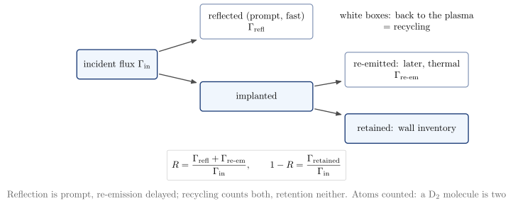
vaft.diagram.plasma_wall_interaction_recycling()Reflection, re-emission and retention as flux bookkeeping.
vaft.diagram.plasma_wall_interaction_recycling(*, labels=True)Show source vaft/diagram/_pwi.py, lines 264–297
def plasma_wall_interaction_recycling(*, labels: bool = True) -> Diagram:
r"""Reflection, re-emission and retention as flux bookkeeping.
The incident flux splits into a promptly reflected part and an implanted
part; the implanted part is either re-emitted later (diffusion,
recombination, desorption) or retained as wall inventory. Recycling is
reflection plus re-emission (``recycling_coefficient``); retention is the
rest; a wall releasing an earlier inventory returns more than it
receives ($R > 1$), a saturated one about as much ($R \\to 1$).
"""
labels = _check_labels(labels)
items: List = []
incident = box(1.8, 0.0, 3.0, 1.1, "incident flux $\\Gamma_\\mathrm{in}$", role="flux:incident", latex=True)
reflected = box(7.0, 1.6, 4.2, 1.3, "reflected (prompt, fast)\\\\ $\\Gamma_\\mathrm{refl}$", role="flux:reflected",
latex=True, style="concept leaf")
implanted = box(7.0, -1.2, 4.2, 1.1, "implanted", role="flux:implanted", latex=True)
reemitted = box(12.6, -0.2, 4.6, 1.3, "re-emitted: later, thermal\\\\ $\\Gamma_\\mathrm{re\\text{-}em}$",
role="flux:reemitted", latex=True, style="concept leaf")
retained = box(12.6, -2.4, 4.6, 1.1, "retained: wall inventory", role="flux:retained", latex=True)
for b in (incident, reflected, implanted, reemitted, retained):
items += list(b.items)
for a, b in ((incident, reflected), (incident, implanted), (implanted, reemitted), (implanted, retained)):
items.append(connector(a, b, role="edge"))
if labels:
items += [
Label((12.6, 1.6), "white boxes: back to the plasma\\\\ = recycling", "small label,align=center",
anchor="center", role="recycling"),
Label((7.0, -3.2), f"$\\displaystyle {formula_equation(recycling_coefficient)}$", "formula box",
anchor="north", role="equations"),
_note("Reflection is prompt, re-emission delayed; recycling counts both, retention neither. Atoms "
"counted: a D$_2$ molecule is two", 7.0, -4.6),
]
return Diagram("plasma_wall_interaction_recycling", Scene(tuple(items)),
model={"returned": ("reflected", "re-emitted"), "kept": ("retained",), "imas": IMAS_WALL_PATHS})Formats .svg .tex .pdf the SVG above is committed; build the others locally
import vaft.diagram
d = vaft.diagram.plasma_wall_interaction_recycling()
d.tikz # the TikZ document as text
d.save("plasma_wall_interaction_recycling.svg") # rendered vector image, the canonical artifact; needs latex, dvisvgm
d.save("plasma_wall_interaction_recycling.tex") # the complete TikZ document, the text source
d.save("plasma_wall_interaction_recycling.pdf") # vector PDF; needs pdflatexFormula functions referenced:
pwi.recycling_coefficient
plasma_wall_interaction_energy_partition
1 asset
source
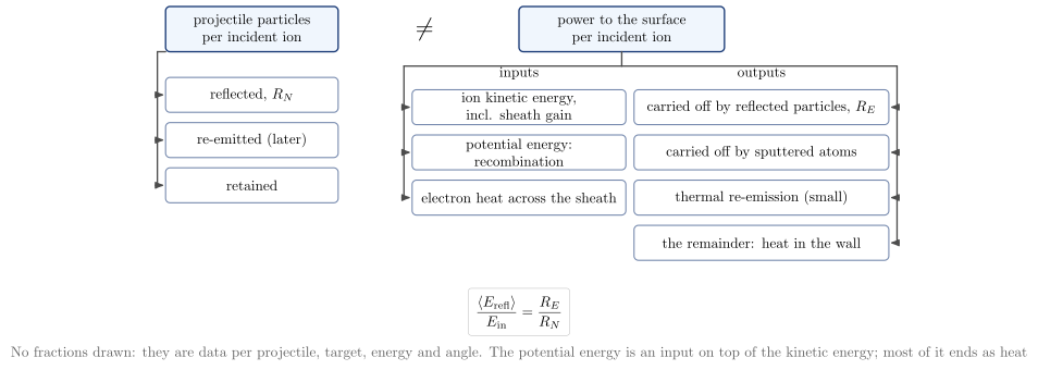
vaft.diagram.plasma_wall_interaction_energy_partition()Particle balance and energy balance, side by side: not the same bookkeeping.
vaft.diagram.plasma_wall_interaction_energy_partition(*, labels=True)Show source vaft/diagram/_pwi.py, lines 300–357
def plasma_wall_interaction_energy_partition(*, labels: bool = True) -> Diagram:
r"""Particle balance and energy balance, side by side: not the same bookkeeping.
Left, where the projectile particles go: reflected ($R_N$), re-emitted,
retained. Right, the power to the surface: its inputs -- ion kinetic
energy including what the sheath adds, the potential energy released when
the ion recombines (and atoms form molecules), and the electrons' heat
across the sheath -- and its outputs: carried off by reflected particles
($R_E$ of the ion kinetic energy), by sputtered atoms and by thermal
re-emission, with the remainder deposited as heat. A surface can return
most particles while keeping most of their energy, $R_E/R_N < 1$
(``mean_reflected_energy_fraction``).
"""
labels = _check_labels(labels)
items: List = []
pb = box(2.5, 0.0, 4.2, 1.1, "projectile particles\\\\ per incident ion", role="balance:particles", latex=True)
eb = box(11.5, 0.0, 5.0, 1.1, "power to the surface\\\\ per incident ion", role="balance:energy", latex=True)
items += list(pb.items) + list(eb.items)
parts_p = ["reflected, $R_N$", "re-emitted (later)", "retained"]
inputs = ["ion kinetic energy, incl. sheath gain", "potential energy: recombination", "electron heat across the sheath"]
outputs = ["carried off by reflected particles, $R_E$", "carried off by sputtered atoms",
"thermal re-emission (small)", "the remainder: heat in the wall"]
def column(x, y0, texts, role, width):
boxes = []
for k, text in enumerate(texts):
b = box(x, y0 - 1.1 * k, width, 0.85, text, role=f"{role}:{k}", latex=True, style="concept leaf")
boxes.append(b)
return boxes
left = column(2.5, -1.6, parts_p, "particles", 4.2)
ins = column(9.0, -1.9, inputs, "energy_in", 5.2)
outs = column(14.9, -1.9, outputs, "energy_out", 6.2)
for b in left + ins + outs:
items += list(b.items)
# a spine from each header to its leaves, so every leaf is connected
for head, leaves, x_spine in ((pb, left, 0.2), (eb, ins, 6.2), (eb, outs, 18.2)):
y_top = head.y - 0.55 if head is pb else -0.9
items.append(Polyline.of([(x_spine, y_top), (x_spine, leaves[-1].y)], "connector line", role="spine"))
for leaf in leaves:
edge = leaf.x - leaf.width / 2 if x_spine < leaf.x else leaf.x + leaf.width / 2
items.append(Arrow((x_spine, leaf.y), (edge, leaf.y), "connector", role="edge"))
items.append(Polyline.of([(6.2, -0.9), (18.2, -0.9)], "connector line", role="spine"))
items.append(Polyline.of([(eb.x, -0.55), (eb.x, -0.9)], "connector line", role="spine"))
items.append(Polyline.of([(pb.x - 2.1, -0.55), (0.2, -0.55)], "connector line", role="spine"))
if labels:
items += [
Label((9.0, -1.35), "inputs", "small label", anchor="south", role="group"),
Label((14.9, -1.35), "outputs", "small label", anchor="south", role="group"),
Label((6.7, 0.0), "$\\neq$", "legend symbol", role="not_equal"),
Label((9.0, -6.3), f"$\\displaystyle {formula_equation(mean_reflected_energy_fraction)}$",
"formula box", anchor="north", role="equations"),
_note("No fractions drawn: they are data per projectile, target, energy and angle. The potential energy "
"is an input on top of the kinetic energy; most of it ends as heat", 9.0, -7.6),
]
return Diagram("plasma_wall_interaction_energy_partition", Scene(tuple(items)),
model={"particles": tuple(parts_p), "energy_in": tuple(inputs), "energy_out": tuple(outputs),
"imas": IMAS_WALL_PATHS})Formats .svg .tex .pdf the SVG above is committed; build the others locally
import vaft.diagram
d = vaft.diagram.plasma_wall_interaction_energy_partition()
d.tikz # the TikZ document as text
d.save("plasma_wall_interaction_energy_partition.svg") # rendered vector image, the canonical artifact; needs latex, dvisvgm
d.save("plasma_wall_interaction_energy_partition.tex") # the complete TikZ document, the text source
d.save("plasma_wall_interaction_energy_partition.pdf") # vector PDF; needs pdflatexFormula functions referenced:
pwi.mean_reflected_energy_fraction
plasma_wall_interaction_reflection_energy
1 asset
source
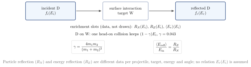
vaft.diagram.plasma_wall_interaction_reflection_energy()Incident energy to reflected energy: two distributions joined by the surface interaction.
vaft.diagram.plasma_wall_interaction_reflection_energy(projectile='D', target='W', *, labels=True)Show source vaft/diagram/_pwi.py, lines 367–408
def plasma_wall_interaction_reflection_energy(projectile="D", target="W", *, labels: bool = True) -> Diagram:
r"""Incident energy to reflected energy: two distributions joined by the surface interaction.
An incident state $f_i(E_i)$ meets the target; a reflected state
$f_r(E_r)$ leaves it. The only kinematic fact drawn is the binary-collision
limit: a projectile backscattered by one head-on collision keeps
$(1 - \gamma)E_i$, with $\gamma$ from
``binary_collision_energy_transfer_factor`` for the pair. $R_N(E_i)$,
$R_E(E_i)$ and $\langle E_r\rangle(E_i)$ are the enrichment slots of
#1047 level 2; they are data and stay empty here, so no functional
relation between $E_i$ and $E_r$ is drawn.
"""
labels = _check_labels(labels)
p, t = _species(projectile), _species(target)
if p not in MASS_U or t not in MASS_U:
raise ValueError(f"no mass tabulated here for {p if p not in MASS_U else t}")
gamma = float(binary_collision_energy_transfer_factor(MASS_U[p], MASS_U[t]))
incident = box(0.0, 0.0, 4.4, 1.6, f"incident {p}\\\\ $f_i(E_i)$", role="state:incident", latex=True)
surface = box(6.6, 0.0, 4.0, 1.6, f"surface interaction\\\\ target {t}", role="surface", latex=True,
style="concept leaf")
reflected = box(13.2, 0.0, 4.4, 1.6, f"reflected {p}\\\\ $f_r(E_r)$", role="state:reflected", latex=True)
items: List = []
for b in (incident, surface, reflected):
items += list(b.items)
items += [connector(incident, surface, role="edge"), connector(surface, reflected, role="edge")]
if labels:
items += [
Label((6.6, -1.1), "enrichment slots (data, not drawn): $R_N(E_i)$, $R_E(E_i)$, "
"$\\langle E_r\\rangle(E_i)$", "small label", anchor="north", role="enrichment"),
Label((6.6, -1.75), f"{p} on {t}: one head-on collision keeps $(1-\\gamma)E_i$, $\\gamma = {gamma:.3f}$",
"small label", anchor="north", role="kinematics"),
Label((3.3, -2.6), f"$\\displaystyle {formula_equation(binary_collision_energy_transfer_factor)}$",
"formula box", anchor="north", role="equations"),
Label((10.3, -2.6), f"$\\displaystyle {formula_equation(mean_reflected_energy_fraction)}$",
"formula box", anchor="north", role="equations"),
_note("Particle reflection ($R_N$) and energy reflection ($R_E$) are different data per projectile, "
"target, energy and angle; no relation $E_r(E_i)$ is assumed", 6.6, -4.2),
]
return Diagram("plasma_wall_interaction_reflection_energy", Scene(tuple(items)),
model={"projectile": p, "target": t, "gamma": gamma,
"enrichment": {"R_N(E_i)": None, "R_E(E_i)": None, "<E_r>(E_i)": None},
"imas": IMAS_WALL_PATHS})Formats .svg .tex .pdf the SVG above is committed; build the others locally
import vaft.diagram
d = vaft.diagram.plasma_wall_interaction_reflection_energy()
d.tikz # the TikZ document as text
d.save("plasma_wall_interaction_reflection_energy.svg") # rendered vector image, the canonical artifact; needs latex, dvisvgm
d.save("plasma_wall_interaction_reflection_energy.tex") # the complete TikZ document, the text source
d.save("plasma_wall_interaction_reflection_energy.pdf") # vector PDF; needs pdflatexFormula functions referenced:
pwi.binary_collision_energy_transfer_factor, pwi.mean_reflected_energy_fraction
plasma_wall_interaction_angle_dependence
1 asset
source
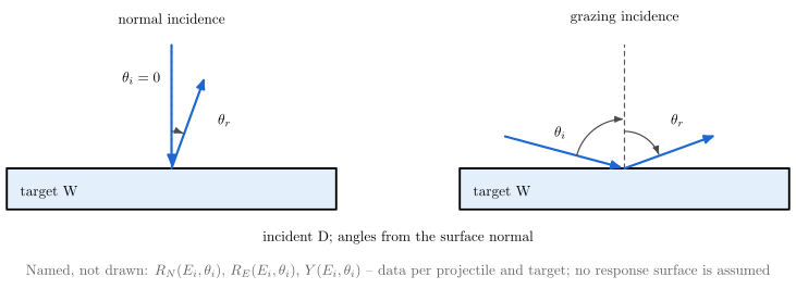
vaft.diagram.plasma_wall_interaction_angle_dependence()Normal and grazing incidence side by side, angles measured from the surface normal.
vaft.diagram.plasma_wall_interaction_angle_dependence(projectile='D', target='W', *, labels=True)Show source vaft/diagram/_pwi.py, lines 411–459
def plasma_wall_interaction_angle_dependence(projectile="D", target="W", *, labels: bool = True) -> Diagram:
r"""Normal and grazing incidence side by side, angles measured from the surface normal.
The same projectile reaches the same target at $\theta_i = 0$ (normal) and
near $90^\circ$ (grazing); the reflected particle leaves at $\theta_r$.
The response at each angle -- $R_N(E_i, \theta_i)$, $R_E(E_i, \theta_i)$,
$Y(E_i, \theta_i)$ -- is data and is named, not drawn: no response
surface is assumed.
"""
labels = _check_labels(labels)
p, t = _species(projectile), _species(target)
items: List = []
panels = {"normal": (0.0, 0.0, math.radians(20.0)), "grazing": (11.0, math.radians(75.0), math.radians(70.0))}
for name, (x0, th_in, th_out) in panels.items():
items += [it for it in _wall(x0, x0 + 8.0, 1.0)]
hit = (x0 + 4.0, 0.0)
L_in, L_out = 3.0, 2.4
start = (hit[0] - L_in * math.sin(th_in), L_in * math.cos(th_in))
end = (hit[0] + L_out * math.sin(th_out), L_out * math.cos(th_out))
items += [Polyline.of([hit, (hit[0], 3.0)], "approx", role=f"normal:{name}"),
Arrow(start, hit, "drift ion", role=f"incident:{name}"),
Arrow(hit, end, "drift ion", role=f"reflected:{name}"),
_arc(hit, 0.9, 0.0, th_out, f"angle_out:{name}")]
if th_in > 0:
items.append(_arc(hit, 1.2, -th_in, 0.0, f"angle_in:{name}"))
if labels:
items += [
Label((hit[0], 3.4), f"{name} incidence", "small label", anchor="south", role=f"title:{name}"),
Label((x0 + 0.2, -0.3), f"target {t}", "small label", anchor="north west", role=f"wall:{name}"),
Label((hit[0] + 1.0, 0.9), "$\\theta_r$", "small label", anchor="south west",
role=f"angle_out:{name}"),
]
if th_in > 0:
items.append(Label((hit[0] - 1.3, 0.6), "$\\theta_i$", "small label", anchor="south east",
role=f"angle_in:{name}"))
else:
items.append(Label((hit[0] - 0.15, 2.2), "$\\theta_i = 0$", "small label", anchor="east",
role=f"angle_in:{name}"))
if labels:
items += [
Label((9.5, -1.4), f"incident {p}; angles from the surface normal", "small label", anchor="north",
role="convention"),
_note("Named, not drawn: $R_N(E_i,\\theta_i)$, $R_E(E_i,\\theta_i)$, $Y(E_i,\\theta_i)$ -- data per "
"projectile and target; no response surface is assumed", 9.5, -2.2),
]
return Diagram("plasma_wall_interaction_angle_dependence", Scene(tuple(items)),
model={"projectile": p, "target": t, "angles": "from the surface normal",
"enrichment": {"R_N(E_i,theta_i)": None, "R_E(E_i,theta_i)": None, "Y(E_i,theta_i)": None},
"imas": IMAS_WALL_PATHS})Formats .svg .tex .pdf the SVG above is committed; build the others locally
import vaft.diagram
d = vaft.diagram.plasma_wall_interaction_angle_dependence()
d.tikz # the TikZ document as text
d.save("plasma_wall_interaction_angle_dependence.svg") # rendered vector image, the canonical artifact; needs latex, dvisvgm
d.save("plasma_wall_interaction_angle_dependence.tex") # the complete TikZ document, the text source
d.save("plasma_wall_interaction_angle_dependence.pdf") # vector PDF; needs pdflatexplasma_wall_interaction_sputtering_threshold
1 asset
source
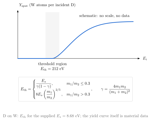
vaft.diagram.plasma_wall_interaction_sputtering_threshold(surface_binding_energy=8.68)Sputtering yield against incident energy: a threshold, drawn qualitatively.
vaft.diagram.plasma_wall_interaction_sputtering_threshold(projectile='D', target='W', surface_binding_energy=None, *, labels=True)Show source vaft/diagram/_pwi.py, lines 462–506
def plasma_wall_interaction_sputtering_threshold(projectile="D", target="W",
surface_binding_energy: Optional[float] = None, *,
labels: bool = True) -> Diagram:
r"""Sputtering yield against incident energy: a threshold, drawn qualitatively.
A schematic $Y(E_i)$: zero below a threshold, rising above it, levelling
off. The axes carry no scale and the curve no data -- it shows that a
threshold exists, not where it is or how steeply the yield rises. A value
for $E_\mathrm{th}$ is printed only when ``surface_binding_energy`` is
given, from Bohdansky's fit (``sputtering_threshold_bohdansky``).
"""
labels = _check_labels(labels)
p, t = _species(projectile), _species(target)
if p not in MASS_U or t not in MASS_U:
raise ValueError(f"no mass tabulated here for {p if p not in MASS_U else t}")
E_th = None
if surface_binding_energy is not None:
E_th = float(sputtering_threshold_bohdansky(surface_binding_energy, MASS_U[p], MASS_U[t]))
x_th = 3.0
x = np.linspace(0.0, 10.0, 200)
y = 3.2 * (1.0 - np.exp(-(np.clip(x - x_th, 0.0, None) / 2.4) ** 1.6)) # schematic shape only: 0 below x_th
items: List = [
Polyline.of([(x_th - 0.6, 0.0), (x_th + 0.6, 0.0), (x_th + 0.6, 4.0), (x_th - 0.6, 4.0)], "concept band",
role="threshold_region", closed=True),
Arrow((0.0, 0.0), (10.6, 0.0), "axis", role="axis:x"),
Arrow((0.0, 0.0), (0.0, 4.2), "axis", role="axis:y"),
Polyline.of(np.stack([x, y], -1), "crest", role="schematic_yield"),
]
if labels:
items += [
Label((10.7, 0.0), "$E_i$", "small label", anchor="west", role="axis:x"),
Label((0.0, 4.3), f"$Y_\\mathrm{{sput}}$ ({t} atoms per incident {p})", "small label", anchor="south west",
role="axis:y"),
Label((x_th, -0.2), "threshold region" + (f"\\\\ $E_\\mathrm{{th}} = {E_th:.0f}$ eV" if E_th else ""),
"small label,align=center", anchor="north", role="threshold"),
Label((7.5, 3.4), "schematic: no scale, no data", "small label", anchor="south", role="schematic"),
Label((5.0, -1.6), f"$\\displaystyle {formula_equation(sputtering_threshold_bohdansky)}$", "formula box",
anchor="north", role="equations"),
_note(f"{p} on {t}: " + (f"$E_\\mathrm{{th}}$ for the supplied $E_s = {surface_binding_energy:g}$ eV"
if E_th else "$E_\\mathrm{th}$ needs the surface binding energy $E_s$ (not assumed)")
+ "; the yield curve itself is material data", 5.0, -4.7),
]
return Diagram("plasma_wall_interaction_sputtering_threshold", Scene(tuple(items)),
model={"projectile": p, "target": t, "threshold_eV": E_th, "schematic": True,
"enrichment": {"Y(E_i)": None}, "imas": IMAS_WALL_PATHS})Formats .svg .tex .pdf the SVG above is committed; build the others locally
import vaft.diagram
d = vaft.diagram.plasma_wall_interaction_sputtering_threshold(surface_binding_energy=8.68)
d.tikz # the TikZ document as text
d.save("plasma_wall_interaction_sputtering_threshold.svg") # rendered vector image, the canonical artifact; needs latex, dvisvgm
d.save("plasma_wall_interaction_sputtering_threshold.tex") # the complete TikZ document, the text source
d.save("plasma_wall_interaction_sputtering_threshold.pdf") # vector PDF; needs pdflatexFormula functions referenced:
pwi.sputtering_threshold_bohdansky
plasma_wall_interaction_particle_balance
1 asset
source
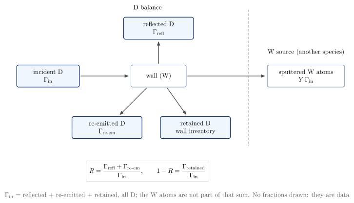
vaft.diagram.plasma_wall_interaction_particle_balance()The projectile’s particle balance, and the target-material source beside it, not inside it.
vaft.diagram.plasma_wall_interaction_particle_balance(projectile='D', target='W', *, labels=True)Show source vaft/diagram/_pwi.py, lines 509–547
def plasma_wall_interaction_particle_balance(projectile="D", target="W", *, labels: bool = True) -> Diagram:
r"""The projectile's particle balance, and the target-material source beside it, not inside it.
Incident projectiles leave the wall reflected, re-emitted or not at all
(retained); those three close the projectile balance, and recycling is the
first two (``recycling_coefficient``). Sputtering creates a second species
-- target atoms -- whose source is drawn apart: a sputtered tungsten atom
is not a branch of the deuterium balance.
"""
labels = _check_labels(labels)
p, t = _species(projectile), _species(target)
incident = box(0.0, 0.0, 3.4, 1.2, f"incident {p}\\\\ $\\Gamma_\\mathrm{{in}}$", role="flux:incident", latex=True)
wall = box(6.0, 0.0, 3.0, 1.2, f"wall ({t})", role="wall", latex=True, style="concept leaf")
reflected = box(6.0, 2.6, 3.8, 1.2, f"reflected {p}\\\\ $\\Gamma_\\mathrm{{refl}}$", role="flux:reflected",
latex=True)
reemitted = box(3.2, -2.8, 3.8, 1.2, f"re-emitted {p}\\\\ $\\Gamma_\\mathrm{{re\\text{{-}}em}}$",
role="flux:reemitted", latex=True)
retained = box(8.0, -2.8, 3.8, 1.2, f"retained {p}\\\\ wall inventory", role="flux:retained", latex=True)
sputtered = box(14.0, 0.0, 4.2, 1.2, f"sputtered {t} atoms\\\\ $Y\\,\\Gamma_\\mathrm{{in}}$",
role="flux:sputtered", latex=True, style="concept leaf")
items: List = []
for b in (incident, wall, reflected, reemitted, retained, sputtered):
items += list(b.items)
for a, b in ((incident, wall), (wall, reflected), (wall, reemitted), (wall, retained), (wall, sputtered)):
items.append(connector(a, b, role=f"edge:{b.items[0].role}"))
# the projectile balance is everything left of the dashed line; the target source is to its right
items.append(Polyline.of([(10.9, 3.6), (10.9, -3.8)], "approx", role="species_boundary"))
if labels:
items += [
Label((5.4, 3.5), f"{p} balance", "small label", anchor="south", role="group:projectile"),
Label((14.0, 1.0), f"{t} source (another species)", "small label", anchor="south", role="group:target"),
Label((5.4, -4.6), f"$\\displaystyle {formula_equation(recycling_coefficient)}$", "formula box",
anchor="north", role="equations"),
_note(f"$\\Gamma_\\mathrm{{in}}$ = reflected + re-emitted + retained, all {p}; the {t} atoms are not "
f"part of that sum. No fractions drawn: they are data", 7.0, -6.2),
]
return Diagram("plasma_wall_interaction_particle_balance", Scene(tuple(items)),
model={"projectile": p, "target": t, "projectile_balance": ("reflected", "re-emitted", "retained"),
"target_source": ("sputtered",), "imas": IMAS_WALL_PATHS})Formats .svg .tex .pdf the SVG above is committed; build the others locally
import vaft.diagram
d = vaft.diagram.plasma_wall_interaction_particle_balance()
d.tikz # the TikZ document as text
d.save("plasma_wall_interaction_particle_balance.svg") # rendered vector image, the canonical artifact; needs latex, dvisvgm
d.save("plasma_wall_interaction_particle_balance.tex") # the complete TikZ document, the text source
d.save("plasma_wall_interaction_particle_balance.pdf") # vector PDF; needs pdflatexFormula functions referenced:
pwi.recycling_coefficient
plasma_wall_interaction_surface_response
1 asset
source
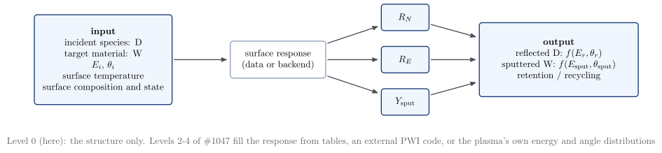
vaft.diagram.plasma_wall_interaction_surface_response()The generic surface-response model: what a PWI backend takes in and returns.
vaft.diagram.plasma_wall_interaction_surface_response(projectile='D', target='W', *, labels=True)Show source vaft/diagram/_pwi.py, lines 550–586
def plasma_wall_interaction_surface_response(projectile="D", target="W", *, labels: bool = True) -> Diagram:
r"""The generic surface-response model: what a PWI backend takes in and returns.
Inputs (species, material, incident energy and angle, surface temperature,
composition and state) feed a surface response that returns the particle
and energy reflection coefficients and the sputtering yield, and from them
the reflected and sputtered distributions and the retained/recycled split.
This is the extension point of #1047 levels 2-4: tabulated data or an
external code fills the response; at level 0 it is empty.
"""
labels = _check_labels(labels)
p, t = _species(projectile), _species(target)
inputs = (f"incident species: {p}", f"target material: {t}", "$E_i$, $\\theta_i$", "surface temperature",
"surface composition and state")
coefficients = ("$R_N$", "$R_E$", "$Y_\\mathrm{sput}$")
outputs = (f"reflected {p}: $f(E_r, \\theta_r)$", f"sputtered {t}: $f(E_\\mathrm{{sput}}, \\theta_\\mathrm{{sput}})$",
"retention / recycling")
inp = box(0.0, 0.0, 5.2, 3.4, "\\textbf{input}\\\\ " + "\\\\ ".join(inputs), role="inputs", latex=True)
response = box(6.6, 0.0, 3.6, 1.4, "surface response\\\\ (data or backend)", role="response", latex=True,
style="concept leaf")
coef = [box(11.4, 1.6 - 1.6 * k, 1.8, 1.0, c, role=f"coefficient:{k}", latex=True) for k, c in
enumerate(coefficients)]
out = box(17.2, 0.0, 6.0, 2.8, "\\textbf{output}\\\\ " + "\\\\ ".join(outputs), role="outputs", latex=True)
items: List = []
for b in (inp, response, *coef, out):
items += list(b.items)
items.append(connector(inp, response, role="edge"))
for c in coef:
items += [connector(response, c, role="edge"), connector(c, out, role="edge")]
if labels:
items += [
_note("Level 0 (here): the structure only. Levels 2-4 of \\#1047 fill the response from tables, an "
"external PWI code, or the plasma's own energy and angle distributions", 8.6, -2.8),
]
return Diagram("plasma_wall_interaction_surface_response", Scene(tuple(items)),
model={"projectile": p, "target": t, "inputs": inputs, "coefficients": ("R_N", "R_E", "Y_sput"),
"outputs": outputs, "backend": None, "imas": IMAS_WALL_PATHS})Formats .svg .tex .pdf the SVG above is committed; build the others locally
import vaft.diagram
d = vaft.diagram.plasma_wall_interaction_surface_response()
d.tikz # the TikZ document as text
d.save("plasma_wall_interaction_surface_response.svg") # rendered vector image, the canonical artifact; needs latex, dvisvgm
d.save("plasma_wall_interaction_surface_response.tex") # the complete TikZ document, the text source
d.save("plasma_wall_interaction_surface_response.pdf") # vector PDF; needs pdflatexSpectroscopy and ionization concept diagrams, with progressive metadata
Module vaft.diagram._spectroscopy
spectroscopy_ionization_stages
1 asset
source

vaft.diagram.spectroscopy_ionization_stages(term='C III')All ionization stages of an element, the one a term names highlighted.
vaft.diagram.spectroscopy_ionization_stages(term='C III', *, labels=True)Show source vaft/diagram/_spectroscopy.py, lines 85–138
def spectroscopy_ionization_stages(term="C III", *, labels: bool = True) -> Diagram:
r"""All ionization stages of an element, the one a term names highlighted.
``term`` is anything :mod:`vaft.data.spectroscopy` parses -- ``"C III"``,
``"C2+"``, ``"carbon"``, ``"CIII_1909"``. Stage $s$ is charge $s - 1$
(C III is C$^{2+}$); hydrogen isotopes are hydrogen with a mass number,
not elements of their own. Arrows: ionization to the right, recombination
to the left. Elements with more than twelve stages show the first ten and
the fully stripped ion. Semantic only: no atomic data are needed.
"""
labels = _check_labels(labels)
ident = identity(term)
element = "H" if ident.species.element in ("D", "T") else ident.species.element
Z = ATOMIC_NUMBERS[element]
selected = ident.species.ionization_stage
if selected is None and ident.series is not None:
selected = 1 # a hydrogen series member is a line of the neutral atom
stages = list(range(1, Z + 2))
if len(stages) > 12:
head = stages[:9]
if selected is not None and selected > 9 and selected < Z + 1:
stages = head + [None, selected, None, Z + 1] # keep the named stage in view
else:
stages = head + [None, Z + 1]
items: List = []
boxes = []
for k, stage in enumerate(stages):
x = 1.3 + 2.9 * k
if stage is None:
items.append(Label((x, 0.0), "$\\cdots$", "label", role="ellipsis"))
boxes.append(None)
continue
b = box(x, 0.0, 2.1, 1.3, _stage_text(element, stage), role=f"stage:{stage}", latex=True)
items += list(b.items)
if stage == selected: # the stage the term names: outlined in red
items.append(Polyline.of([(x - 1.15, -0.75), (x + 1.15, -0.75), (x + 1.15, 0.75), (x - 1.15, 0.75)],
"trough", role="selected", closed=True))
boxes.append(b)
for a, b in zip(boxes[:-1], boxes[1:]):
if a is None or b is None:
continue
items.append(Arrow((a.x + 1.1, 0.3), (b.x - 1.1, 0.3), "connector", role="ionization"))
items.append(Arrow((b.x - 1.1, -0.3), (a.x + 1.1, -0.3), "connector", role="recombination"))
if labels:
mass = ident.species.mass_number
name = {1: "hydrogen", 2: "deuterium", 3: "tritium"}.get(mass, element) if element == "H" else element
items += [
Label((1.3 + 1.45 * (len(stages) - 1), 1.1), f"{name}: ionization stages (upper arrows: ionization, "
"lower: recombination)", "label", anchor="south", role="title"),
_note(f"Stage $s$ = charge $s - 1$; highlighted: {term!s} as parsed by vaft.data.spectroscopy. Semantic "
"only: no atomic data used", 1.3 + 1.45 * (len(stages) - 1), -1.1),
]
return Diagram("spectroscopy_ionization_stages", Scene(tuple(items)),
model={"identity": ident, "element": element, "stages": stages, "selected": selected})Formats .svg .tex .pdf the SVG above is committed; build the others locally
import vaft.diagram
d = vaft.diagram.spectroscopy_ionization_stages(term='C III')
d.tikz # the TikZ document as text
d.save("spectroscopy_ionization_stages.svg") # rendered vector image, the canonical artifact; needs latex, dvisvgm
d.save("spectroscopy_ionization_stages.tex") # the complete TikZ document, the text source
d.save("spectroscopy_ionization_stages.pdf") # vector PDF; needs pdflatexspectroscopy_transitions
2 assets
source
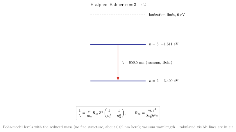
vaft.diagram.spectroscopy_transitions(term='H-alpha')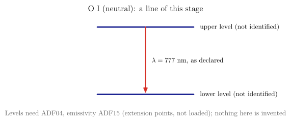
vaft.diagram.spectroscopy_transitions(term='OI_7770')The transition behind one emission term, with no more metadata than exists.
vaft.diagram.spectroscopy_transitions(term='H-alpha', *, labels=True)Show source vaft/diagram/_spectroscopy.py, lines 148–223
def spectroscopy_transitions(term="H-alpha", *, labels: bool = True) -> Diagram:
r"""The transition behind one emission term, with no more metadata than exists.
A hydrogen series member (``"H-alpha"``, ``"D-beta"``, ``"H-alpha_6563"``)
is a Balmer line: its levels $n = 3, 4, \ldots \to 2$ and vacuum wavelength
are the Bohr-model values (``hydrogenic_energy_level``,
``hydrogenic_transition_wavelength``, with the isotope's reduced mass;
an unspecified isotope is taken as protium). Any
other line (``"OI_7770"``, ``"C III"``) is drawn as an unnamed upper and
lower level of its ionization stage, with the wavelength only if its label
declares one; level identities would need ADF04, photon emissivities
ADF15.
"""
labels = _check_labels(labels)
ident = identity(term)
element = "H" if ident.species.element in ("D", "T") else ident.species.element
stage = ident.species.ionization_stage
if stage is not None and stage == ATOMIC_NUMBERS[element] + 1:
raise ValueError(f"{term!r} is a fully stripped ion: it has no bound levels and emits no lines")
pair = _balmer(ident)
if pair is None and element == "H":
raise ValueError(f"{term!r} names hydrogen but no line: pass a series member such as 'H-alpha' or 'D-beta'")
items: List = []
model = {"identity": ident, "hydrogenic": pair is not None}
if pair is not None:
n_u, n_l = pair
assumed = ident.species.mass_number is None
mass = ident.species.mass_number or 1 # an unspecified hydrogen isotope is taken as protium
model["source"] = "vaft.formula.atomic: Bohr model with the reduced mass" + (", protium assumed" if assumed else "")
E_u, E_l = hydrogenic_energy_level(n_u, 1, mass), hydrogenic_energy_level(n_l, 1, mass)
lam = hydrogenic_transition_wavelength(n_u, n_l, 1, mass)
scale = 6.0 / abs(E_l)
y_u, y_l = 6.0 + scale * E_u + 2.0, 6.0 + scale * E_l + 2.0
items += [Polyline.of([(0.0, y_u), (5.0, y_u)], "boundary", role="level:upper"),
Polyline.of([(0.0, y_l), (5.0, y_l)], "boundary", role="level:lower"),
Polyline.of([(0.0, 8.0), (5.0, 8.0)], "approx", role="ionization_limit"),
Arrow((2.5, y_u), (2.5, y_l), "drift", role="transition")]
model.update({"n_upper": n_u, "n_lower": n_l, "E_upper_eV": E_u, "E_lower_eV": E_l, "wavelength_m": lam})
if labels:
items += [Label((5.2, y_u), f"$n = {n_u}$, ${E_u:.3f}$ eV", "small label", anchor="west", role="level"),
Label((5.2, y_l), f"$n = {n_l}$, ${E_l:.3f}$ eV", "small label", anchor="west", role="level"),
Label((5.2, 8.0), "ionization limit, 0 eV", "small label", anchor="west", role="level"),
Label((2.7, 0.5 * (y_u + y_l)), f"$\\lambda = {lam * 1e9:.1f}$ nm (vacuum, Bohr)", "small label",
anchor="west", role="wavelength")]
declared = ident.wavelength_angstrom
if declared:
items.append(Label((2.7, 0.5 * (y_u + y_l) - 0.5), f"label declares {declared / 10:g} nm (air, by convention)",
"small label", anchor="west", role="wavelength_declared"))
title = (f"{format_species(ident.species)}-{ident.series}: Balmer $n = {n_u} \\to {n_l}$"
+ (" (protium assumed)" if assumed else ""))
items += [Label((2.5, 8.6), title, "label", anchor="south", role="title"),
Label((2.5, -0.3), f"$\\displaystyle {formula_equation(hydrogenic_transition_wavelength)}$",
"formula box", anchor="north", role="equations")]
else:
items += [Polyline.of([(0.0, 5.0), (5.0, 5.0)], "boundary", role="level:upper"),
Polyline.of([(0.0, 1.5), (5.0, 1.5)], "boundary", role="level:lower"),
Arrow((2.5, 5.0), (2.5, 1.5), "drift", role="transition")]
lam = ident.wavelength_angstrom
model["wavelength_m"] = lam * 1e-10 if lam else None
model["source"] = "the IMAS processed_line label" if lam else None
if labels:
stage = ident.species.ionization_stage
who = format_species(ident.species)
items += [Label((5.2, 5.0), "upper level (not identified)", "small label", anchor="west", role="level"),
Label((5.2, 1.5), "lower level (not identified)", "small label", anchor="west", role="level"),
Label((2.7, 3.25), f"$\\lambda = {lam / 10:g}$ nm, as declared" if lam else
"$\\lambda$ not declared", "small label", anchor="west", role="wavelength"),
Label((2.5, 5.6), f"{who}" + ((f" (charge {charge_state_of(stage)}+)" if charge_state_of(stage)
else " (neutral)") if stage else "")
+ ": a line of this stage", "label", anchor="south", role="title"),
_note("Levels need ADF04, emissivity ADF15 (extension points, not loaded); nothing here is "
"invented", 2.5, 0.8)]
if labels and pair is not None:
items.append(_note("Bohr-model levels with the reduced mass (no fine structure, about 0.02 nm here); vacuum "
"wavelength -- tabulated visible lines are in air", 2.5, -1.9))
return Diagram("spectroscopy_transitions", Scene(tuple(items)), model=model)Formats .svg .tex .pdf the SVG above is committed; build the others locally
import vaft.diagram
d = vaft.diagram.spectroscopy_transitions(term='H-alpha')
d.tikz # the TikZ document as text
d.save("spectroscopy_transitions_h_alpha.svg") # rendered vector image, the canonical artifact; needs latex, dvisvgm
d.save("spectroscopy_transitions_h_alpha.tex") # the complete TikZ document, the text source
d.save("spectroscopy_transitions_h_alpha.pdf") # vector PDF; needs pdflatexFormula functions referenced:
atomic.hydrogenic_energy_level, atomic.hydrogenic_transition_wavelength
spectroscopy_energy_levels
1 asset
source
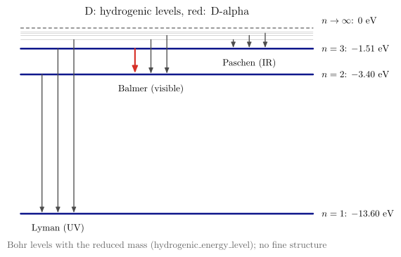
vaft.diagram.spectroscopy_energy_levels(term='D-alpha')The hydrogenic level ladder, with the Lyman, Balmer and Paschen series.
vaft.diagram.spectroscopy_energy_levels(term='H-alpha', *, n_max=7, labels=True)Show source vaft/diagram/_spectroscopy.py, lines 226–280
def spectroscopy_energy_levels(term="H-alpha", *, n_max: int = 7, labels: bool = True) -> Diagram:
r"""The hydrogenic level ladder, with the Lyman, Balmer and Paschen series.
Levels $n = 1\ldots$ ``n_max`` of ``hydrogenic_energy_level`` for the
term's isotope, drawn to scale in energy; downward arrows for the first
members of the Lyman ($\to 1$, UV), Balmer ($\to 2$, visible) and Paschen
($\to 3$, IR) series, the term's own transition highlighted. Hydrogenic
only: many-electron level structure needs ADF04 and raises here.
"""
labels = _check_labels(labels)
ident = identity(term)
if ident.species.element not in ("H", "D", "T"):
raise ValueError(f"{term!r} is not hydrogenic: its levels need OPEN-ADAS ADF04 data, not loaded here")
if ident.species.ionization_stage not in (None, 1):
raise ValueError(f"{term!r} is a bare nucleus: it has no bound levels")
if isinstance(n_max, bool) or not isinstance(n_max, int) or not 4 <= n_max <= 10:
raise ValueError(f"n_max must be an integer from 4 to 10, not {n_max!r}")
mass = ident.species.mass_number or 1 # an unspecified hydrogen isotope is taken as protium
E = {n: hydrogenic_energy_level(n, 1, mass) for n in range(1, n_max + 1)}
scale = 7.0 / abs(E[1])
def y(e):
return 7.5 + scale * e
items: List = [Polyline.of([(0.0, y(0.0)), (11.0, y(0.0))], "approx", role="ionization_limit")]
for n, e in E.items():
items.append(Polyline.of([(0.0, y(e)), (11.0, y(e))], "surface" if n > 3 else "boundary", role=f"level:{n}"))
selected = _balmer(ident)
series = {"Lyman": (1, 0.8), "Balmer": (2, 4.3), "Paschen": (3, 8.0)}
lines = []
for name, (n_l, x0) in series.items():
for k, n_u in enumerate(range(n_l + 1, min(n_l + 4, n_max + 1))):
x = x0 + 0.6 * k
style = "drift" if (n_u, n_l) == selected else "connector"
items.append(Arrow((x, y(E[n_u])), (x, y(E[n_l])), style, role=f"line:{name}:{n_u}"))
lines.append((name, n_u, n_l, hydrogenic_transition_wavelength(n_u, n_l, 1, mass)))
if labels:
for n, e in E.items():
if n <= 3:
items.append(Label((11.2, y(e)), f"$n = {n}$: ${e:.2f}$ eV", "small label", anchor="west",
role="level"))
items.append(Label((11.2, y(0.0) + 0.05), "$n \\to \\infty$: 0 eV", "small label", anchor="south west",
role="level"))
for name, (n_l, x0) in series.items():
band = {"Lyman": "UV", "Balmer": "visible", "Paschen": "IR"}[name]
items.append(Label((x0 + 0.6, y(E[n_l]) - 0.25), f"{name} ({band})", "small label", anchor="north",
role="series"))
items += [Label((5.5, y(0.0) + 0.3), f"{format_species(ident.species)}: hydrogenic levels"
+ (f", red: {ident.label}" if selected else ""), "label", anchor="south", role="title"),
_note("Bohr levels with the reduced mass (hydrogenic\\_energy\\_level); no fine structure", 5.5,
y(E[1]) - 0.9)]
return Diagram("spectroscopy_energy_levels", Scene(tuple(items)),
model={"identity": ident, "levels": E, "lines": lines, "selected": selected,
"source": "vaft.formula.atomic: Bohr model with the reduced mass"
+ (", protium assumed" if ident.species.mass_number is None else "")})Formats .svg .tex .pdf the SVG above is committed; build the others locally
import vaft.diagram
d = vaft.diagram.spectroscopy_energy_levels(term='D-alpha')
d.tikz # the TikZ document as text
d.save("spectroscopy_energy_levels.svg") # rendered vector image, the canonical artifact; needs latex, dvisvgm
d.save("spectroscopy_energy_levels.tex") # the complete TikZ document, the text source
d.save("spectroscopy_energy_levels.pdf") # vector PDF; needs pdflatexFormula functions referenced:
atomic.hydrogenic_energy_level, atomic.hydrogenic_transition_wavelength
spectroscopy_spectrum
1 asset
source
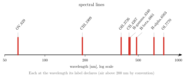
vaft.diagram.spectroscopy_spectrum()Declared spectral lines on a wavelength axis, each at the wavelength its label states.
vaft.diagram.spectroscopy_spectrum(line_labels=None, *, labels=True)Show source vaft/diagram/_spectroscopy.py, lines 283–342
def spectroscopy_spectrum(line_labels: Optional[Sequence[str]] = None, *, labels: bool = True) -> Diagram:
r"""Declared spectral lines on a wavelength axis, each at the wavelength its label states.
``line_labels`` are IMAS ``processed_line.label`` strings or emission
terms (default: the lines the VEST spectrometer declares,
``DECLARED_LABELS``). A line is placed at the wavelength in its label; a
hydrogen series member without one at its computed vacuum wavelength
(dashed); any other line without a wavelength is listed, not placed. The
frames differ: declared wavelengths follow the spectroscopic convention
(air above 200 nm, vacuum below), computed ones are vacuum -- a 0.18 nm
difference at H-alpha, invisible here but not negligible for H/D
separation. Log wavelength axis, 50 to 1000 nm.
"""
labels = _check_labels(labels)
line_labels = tuple(DECLARED_LABELS if line_labels is None else line_labels)
W = 16.0
lo, hi = math.log10(50.0), math.log10(1000.0)
def x(nm):
return W * (math.log10(nm) - lo) / (hi - lo)
items: List = [Arrow((0.0, 0.0), (W + 0.4, 0.0), "chart axis", role="axis")]
for nm in (50, 100, 200, 500, 1000):
items.append(Polyline.of([(x(nm), 0.0), (x(nm), -0.15)], "tick", role="tick"))
if labels:
items.append(Label((x(nm), -0.25), f"{nm}", "small label", anchor="north", role="tick"))
placed, unplaced = [], []
for k, lab in enumerate(line_labels):
ident = identity(lab)
if ident.wavelength_angstrom:
nm, source = ident.wavelength_angstrom / 10.0, "declared"
elif _balmer(ident):
n_u, n_l = _balmer(ident)
nm, source = hydrogenic_transition_wavelength(n_u, n_l, 1, ident.species.mass_number or 1) * 1e9, "computed"
else:
unplaced.append(lab)
continue
placed.append((lab, nm, source))
placed.sort(key=lambda r: r[1])
# label positions: at the line, pushed right to keep 0.6 cm between neighbours, joined by a leader
label_x: List[float] = []
for _lab, nm, _src in placed:
label_x.append(max(x(nm), label_x[-1] + 0.6) if label_x else x(nm))
h = 1.6
for (lab, nm, source), lx in zip(placed, label_x):
items.append(Polyline.of([(x(nm), 0.0), (x(nm), h)], "component real" if source == "declared" else "approx",
role=f"line:{lab}"))
if labels:
items.append(Polyline.of([(x(nm), h), (lx, h + 0.45)], "leader line", role=f"leader:{lab}"))
items.append(Label((lx - 0.05, h + 0.5), lab.replace("_", "\\_"), "small label,rotate=50",
anchor="south west", role=f"line:{lab}"))
if labels:
items += [Label((W / 2, -0.8), "wavelength [nm], log scale", "small label", anchor="north", role="axis"),
Label((W / 2, 4.3), "spectral lines", "label", anchor="south", role="title"),
_note("Each at the wavelength its label declares (air above 200 nm by convention)"
+ ("; dashed: computed vacuum wavelength" if any(src == "computed" for *_x, src in placed)
else "")
+ (f"; not placed (no wavelength): {', '.join(unplaced)}" if unplaced else ""), W / 2, -1.4)]
return Diagram("spectroscopy_spectrum", Scene(tuple(items)),
model={"placed": placed, "unplaced": unplaced, "labels": line_labels})Formats .svg .tex .pdf the SVG above is committed; build the others locally
import vaft.diagram
d = vaft.diagram.spectroscopy_spectrum()
d.tikz # the TikZ document as text
d.save("spectroscopy_spectrum.svg") # rendered vector image, the canonical artifact; needs latex, dvisvgm
d.save("spectroscopy_spectrum.tex") # the complete TikZ document, the text source
d.save("spectroscopy_spectrum.pdf") # vector PDF; needs pdflatexFormula functions referenced:
atomic.hydrogenic_transition_wavelength
Neutral beam injection: the particle lifecycle and the reduced neutral attenuation
Module vaft.diagram._nbi
nbi_particle_lifecycle
1 asset
source
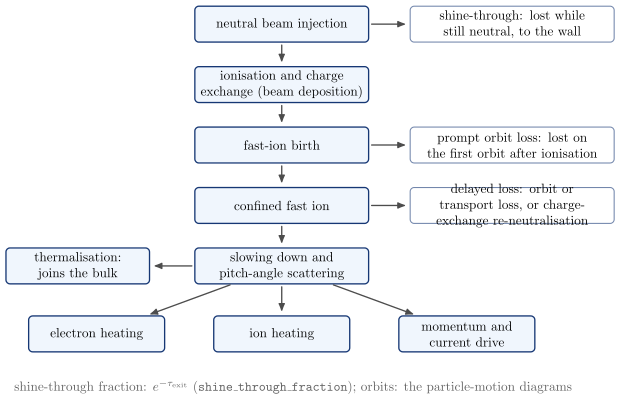
vaft.diagram.nbi_particle_lifecycle()What happens to a beam particle, and the three different ways it is lost.
vaft.diagram.nbi_particle_lifecycle(*, labels=True)Show source vaft/diagram/_nbi.py, lines 50–96
def nbi_particle_lifecycle(*, labels: bool = True) -> Diagram:
r"""What happens to a beam particle, and the three different ways it is lost.
The main path -- injection, ionisation, fast-ion birth, confinement,
slowing down, heating electrons and ions and driving momentum and
current, thermalisation -- runs down the centre; the losses branch to
the right at the stage where they happen: shine-through while still
neutral, prompt orbit loss on the first orbit after ionisation, delayed
loss after the fast ion has been confined for a while. A conceptual
lifecycle, not a NUBEAM power balance.
"""
labels = _check_labels(labels)
t = (lambda s: s) if labels else (lambda s: "")
w, h, lw = 4.6, 0.95, 5.4
nodes = {
"injection": box(0.0, 10.0, w, h, t("neutral beam injection"), role="injection"),
"ionisation": box(0.0, 8.4, w, h, t("ionisation and charge exchange (beam deposition)"), role="ionisation"),
"birth": box(0.0, 6.8, w, h, t("fast-ion birth"), role="birth"),
"confined": box(0.0, 5.2, w, h, t("confined fast ion"), role="confined"),
"slowing": box(0.0, 3.6, w, h, t("slowing down and pitch-angle scattering"), role="slowing_down"),
"electrons": box(-4.9, 1.8, 3.6, h, t("electron heating"), role="electron_heating"),
"ions": box(0.0, 1.8, 3.6, h, t("ion heating"), role="ion_heating"),
"momentum": box(4.9, 1.8, 3.6, h, t("momentum and current drive"), role="momentum_current"),
"thermal": box(-5.4, 3.6, 3.8, h, t("thermalisation: joins the bulk"), role="thermalisation"),
"shine_through": box(6.1, 10.0, lw, h, t("shine-through: lost while still neutral, to the wall"),
style="concept leaf", role="shine_through"),
"prompt_loss": box(6.1, 6.8, lw, h, t("prompt orbit loss: lost on the first orbit after ionisation"),
style="concept leaf", role="prompt_loss"),
"delayed_loss": box(6.1, 5.2, lw, h, t("delayed loss: orbit or transport loss, or charge-exchange "
"re-neutralisation"),
style="concept leaf", role="delayed_loss"),
}
edges = [("injection", "ionisation"), ("ionisation", "birth"), ("birth", "confined"),
("confined", "slowing"), ("slowing", "electrons"), ("slowing", "ions"), ("slowing", "momentum"),
("slowing", "thermal"), ("injection", "shine_through"), ("birth", "prompt_loss"),
("confined", "delayed_loss")]
items: List = []
for node in nodes.values():
items += node.items
for a, b in edges:
items.append(connector(nodes[a], nodes[b], role=f"{a}->{b}"))
if labels:
items.append(Label((0.3, 0.7), "shine-through fraction: $e^{-\\tau_\\mathrm{exit}}$ "
"(\\texttt{shine\\_through\\_fraction}); orbits: the particle-motion diagrams",
"note", anchor="north", role="note"))
return Diagram("nbi_particle_lifecycle", Scene(tuple(items)),
model={"nodes": tuple(nodes), "edges": tuple(edges), "loss_channels": LOSS_CHANNELS})Formats .svg .tex .pdf the SVG above is committed; build the others locally
import vaft.diagram
d = vaft.diagram.nbi_particle_lifecycle()
d.tikz # the TikZ document as text
d.save("nbi_particle_lifecycle.svg") # rendered vector image, the canonical artifact; needs latex, dvisvgm
d.save("nbi_particle_lifecycle.tex") # the complete TikZ document, the text source
d.save("nbi_particle_lifecycle.pdf") # vector PDF; needs pdflatexnbi_neutral_attenuation
1 asset
source
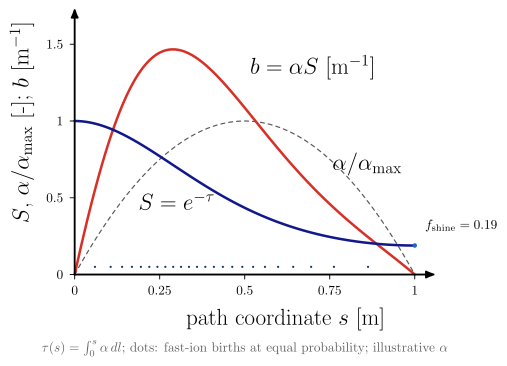
vaft.diagram.nbi_neutral_attenuation()Neutral survival and fast-ion birth along the beam path, and the shine-through at the exit.
vaft.diagram.nbi_neutral_attenuation(*, labels=True)Show source vaft/diagram/_nbi.py, lines 111–157
def nbi_neutral_attenuation(*, labels: bool = True) -> Diagram:
r"""Neutral survival and fast-ion birth along the beam path, and the shine-through at the exit.
For the illustrative $\alpha(s)$ of ``example_attenuation`` (a chord
through a parabolic plasma), the curves are ``neutral_beam_optical_depth``,
``neutral_survival_fraction_from_optical_depth`` and
``beam_birth_probability_density``; the dots are births at equal
probability steps, so their spacing is the birth density; the exit value
of $S$ is ``shine_through_fraction``.
"""
labels = _check_labels(labels)
s = np.linspace(0.0, PATH_LENGTH, 401)
alpha = example_attenuation(s)
tau = neutral_beam_optical_depth(s, alpha)
S = np.asarray(neutral_survival_fraction_from_optical_depth(tau))
b = beam_birth_probability_density(s, alpha)
shine = float(shine_through_fraction(s, alpha))
# births at equal steps of the absorbed fraction 1 - S(s)
absorbed = 1.0 - S
targets = (np.arange(N_BIRTH_MARKERS) + 0.5) / N_BIRTH_MARKERS * absorbed[-1]
s_birth = np.interp(targets, absorbed, s)
chart = Chart(x_range=(0.0, PATH_LENGTH), y_range=(0.0, 1.6))
chart.curves.update({"survival": np.stack([s, S], axis=-1), "birth_density": np.stack([s, b], axis=-1),
"alpha": np.stack([s, alpha / ALPHA_PEAK], axis=-1)})
chart.points["shine_through"] = (PATH_LENGTH, shine)
chart.labels.update({"survival": (0.3, 0.48), "birth": (0.7, 1.35), "alpha": (0.86, 0.72)})
chart.parameters.update({"shine_through_fraction": shine, "tau_exit": float(tau[-1]),
"alpha_peak": ALPHA_PEAK, "path_length": PATH_LENGTH})
scene = render_chart(
chart, x_label="path coordinate $s$ [m]", y_label="$S$, $\\alpha/\\alpha_\\mathrm{max}$ [-]; $b$ [m$^{-1}$]",
curve_styles={"alpha": "approx", "birth_density": "inner solution", "survival": "boundary"},
region_text={"survival": "$S = e^{-\\tau}$", "birth": "$b = \\alpha S$ [m$^{-1}$]",
"alpha": "$\\alpha/\\alpha_\\mathrm{max}$"} if labels else {},
x_ticks=[0.0, 0.25, 0.5, 0.75, 1.0], y_ticks=[0.0, 0.5, 1.0, 1.5],
note=("$\\tau(s) = \\int_0^s \\alpha\\,dl$; dots: fast-ion births at equal probability; "
"illustrative $\\alpha$" if labels else ""),
)
items = list(scene.items)
cm = chart.to_cm
items += [Marker(tuple(cm(np.array([x, 0.05]))), ".", "xpoint", role="birth") for x in s_birth]
exit_point = cm(np.array(chart.points["shine_through"]))
items.append(Marker(tuple(exit_point), "o", "opoint", role="shine_through"))
if labels:
items.append(Label((float(exit_point[0]) + 0.15, float(exit_point[1]) + 0.25),
f"$f_\\mathrm{{shine}} = {shine:.2f}$", "small label", anchor="south west",
role="shine_through"))
return Diagram("nbi_neutral_attenuation", Scene(tuple(items)), model=chart)Formats .svg .tex .pdf the SVG above is committed; build the others locally
import vaft.diagram
d = vaft.diagram.nbi_neutral_attenuation()
d.tikz # the TikZ document as text
d.save("nbi_neutral_attenuation.svg") # rendered vector image, the canonical artifact; needs latex, dvisvgm
d.save("nbi_neutral_attenuation.tex") # the complete TikZ document, the text source
d.save("nbi_neutral_attenuation.pdf") # vector PDF; needs pdflatexFormula functions referenced:
nbi.beam_birth_probability_density, nbi.neutral_beam_optical_depth, nbi.neutral_survival_fraction_from_optical_depth, nbi.shine_through_fraction
Iteration behaviour, branch bifurcation and branch selection: why a solver does not converge
Module vaft.diagram._iteration_dynamics
iteration_behavior
1 asset
source
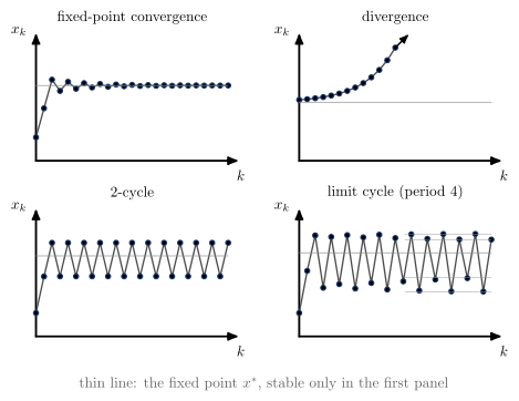
vaft.diagram.iteration_behavior()Four iteration behaviours in one format: state $x_k$ against iteration $k$.
vaft.diagram.iteration_behavior(*, labels=True)Show source vaft/diagram/_iteration_dynamics.py, lines 98–119
def iteration_behavior(*, labels: bool = True) -> Diagram:
r"""Four iteration behaviours in one format: state $x_k$ against iteration $k$.
Computed, not sketched: the logistic map $x_{k+1} = rx_k(1 - x_k)$ at
$r = 2.8$ (convergence to $x^* = 1 - 1/r$), $3.2$ (a 2-cycle) and $3.5$
(a period-4 cycle), and $x_{k+1} = x^* + a(x_k - x^*)$ with $a = 1.3$
(divergence). The thin line is the fixed point $x^*$ in each panel --
it exists in all four, stable only in the first; faint guides mark the
four levels of the period-4 cycle.
"""
labels = _check_labels(labels)
items: List = []
offsets: Dict[str, tuple] = {}
for i, name in enumerate(ITERATION_MAPS):
offsets[name] = ((i % 2) * (_PW + _GAP + 0.6), (1 - i // 2) * (_PH + _GAP + 0.3))
items += Scene(tuple(_panel(name, labels))).transformed(offset=offsets[name]).items
if labels:
items.append(Label((_PW + _GAP / 2 + 0.3, -0.85), "thin line: the fixed point $x^*$, stable only in the first panel",
"note", anchor="north", role="note"))
return Diagram("iteration_behavior", Scene(tuple(items)),
model={"maps": ITERATION_MAPS, "x0": _X0, "orbits": {n: iterate(n) for n in ITERATION_MAPS},
"panel_offsets": offsets})Formats .svg .tex .pdf the SVG above is committed; build the others locally
import vaft.diagram
d = vaft.diagram.iteration_behavior()
d.tikz # the TikZ document as text
d.save("iteration_behavior.svg") # rendered vector image, the canonical artifact; needs latex, dvisvgm
d.save("iteration_behavior.tex") # the complete TikZ document, the text source
d.save("iteration_behavior.pdf") # vector PDF; needs pdflatexbranch_bifurcation
1 asset
source
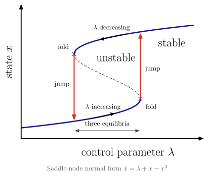
vaft.diagram.branch_bifurcation()Stable and unstable branches, two folds, the jumps and the hysteresis loop.
vaft.diagram.branch_bifurcation(*, labels=True)Show source vaft/diagram/_iteration_dynamics.py, lines 133–194
def branch_bifurcation(*, labels: bool = True) -> Diagram:
r"""Stable and unstable branches, two folds, the jumps and the hysteresis loop.
The saddle-node normal form $\dot x = \lambda + x - x^3$: equilibria on
$\lambda = x^3 - x$, stable where $1 - 3x^2 < 0$ (solid) and unstable
between the folds $x = \pm 1/\sqrt3$ (dashed). Raising $\lambda$ along
the lower branch, the solution disappears at the fold
$\lambda = 2/(3\sqrt3)$ and jumps to the upper branch; lowering it, the
upper branch is followed down to $\lambda = -2/(3\sqrt3)$ -- the path
depends on the direction, the hysteresis. Between the folds three
equilibria coexist.
"""
labels = _check_labels(labels)
x = np.linspace(-1.45, 1.45, 577)
lam = fold_normal_form_equilibria(x)
stable = np.abs(x) > FOLD_X
chart = Chart(x_range=(-1.0, 1.0), y_range=(-1.6, 1.6))
chart.curves.update({"stable_lower": np.stack([lam[x < -FOLD_X], x[x < -FOLD_X]], axis=-1),
"stable_upper": np.stack([lam[x > FOLD_X], x[x > FOLD_X]], axis=-1),
"unstable": np.stack([lam[~stable], x[~stable]], axis=-1)})
# the jump lands on the other stable branch: the third root of x^3 - x - lambda_fold
chart.points.update({"fold_upper": (-FOLD_LAMBDA, FOLD_X), "fold_lower": (FOLD_LAMBDA, -FOLD_X),
"jump_up_to": (FOLD_LAMBDA, 2.0 * FOLD_X), "jump_down_to": (-FOLD_LAMBDA, -2.0 * FOLD_X)})
chart.labels.update({"stable": (0.75, 0.88), "unstable": (0.1, 0.5)})
chart.parameters.update({"fold_lambda": FOLD_LAMBDA, "fold_x": FOLD_X})
scene = render_chart(
chart, x_label="control parameter $\\lambda$", y_label="state $x$",
curve_styles={"stable_lower": "boundary", "stable_upper": "boundary", "unstable": "approx"},
region_text={"stable": "stable", "unstable": "unstable"} if labels else {},
note="Saddle-node normal form $\\dot x = \\lambda + x - x^3$" if labels else "",
)
cm = chart.to_cm
items = list(scene.items)
items += [Marker(tuple(cm(np.array(chart.points[p]))), "x", "xpoint", role="fold") for p in ("fold_upper",
"fold_lower")]
items += [Arrow(tuple(cm(np.array(chart.points["fold_lower"]))), tuple(cm(np.array(chart.points["jump_up_to"]))),
"drift", role="jump_up"),
Arrow(tuple(cm(np.array(chart.points["fold_upper"]))),
tuple(cm(np.array(chart.points["jump_down_to"]))), "drift", role="jump_down")]
# direction of travel along the branches
items += [Arrow(tuple(cm(np.array([-0.2, _branch_x(-0.2, -1)]))),
tuple(cm(np.array([0.1, _branch_x(0.1, -1)]))), "vector", role="increasing"),
Arrow(tuple(cm(np.array([0.2, _branch_x(0.2, 1)]))), tuple(cm(np.array([-0.1, _branch_x(-0.1, 1)]))),
"vector", role="decreasing")]
bistable = [cm(np.array([-FOLD_LAMBDA, -1.4])), cm(np.array([FOLD_LAMBDA, -1.4]))]
items.append(Arrow(tuple(bistable[0]), tuple(bistable[1]), "connector", role="bistable_range", both=True))
if labels:
items += [Label(tuple(cm(np.array(chart.points["fold_lower"])) + [0.15, -0.15]), "fold", "small label",
anchor="north west", role="fold"),
Label(tuple(cm(np.array(chart.points["fold_upper"])) + [-0.15, 0.15]), "fold", "small label",
anchor="south east", role="fold"),
Label(tuple(cm(np.array([-0.05, _branch_x(-0.05, -1)])) + [0.0, 0.2]), "$\\lambda$ increasing",
"small label", anchor="south", role="increasing"),
Label(tuple(cm(np.array([0.05, _branch_x(0.05, 1)])) + [0.0, 0.2]), "$\\lambda$ decreasing",
"small label", anchor="south", role="decreasing"),
Label(tuple((bistable[0] + bistable[1]) / 2 + [0.0, 0.08]), "three equilibria", "small label",
anchor="south", role="bistable_range"),
Label(tuple(cm(np.array([FOLD_LAMBDA, 0.2])) + [0.12, 0.0]), "jump", "small label",
anchor="west", role="jump_up"),
Label(tuple(cm(np.array([-FOLD_LAMBDA, -0.2])) + [-0.12, 0.0]), "jump", "small label",
anchor="east", role="jump_down")]
return Diagram("branch_bifurcation", Scene(tuple(items)), model=chart)Formats .svg .tex .pdf the SVG above is committed; build the others locally
import vaft.diagram
d = vaft.diagram.branch_bifurcation()
d.tikz # the TikZ document as text
d.save("branch_bifurcation.svg") # rendered vector image, the canonical artifact; needs latex, dvisvgm
d.save("branch_bifurcation.tex") # the complete TikZ document, the text source
d.save("branch_bifurcation.pdf") # vector PDF; needs pdflatexbasin_of_attraction
1 asset
source
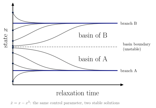
vaft.diagram.basin_of_attraction()Branch selection by the initial condition: two stable solutions at one control parameter.
vaft.diagram.basin_of_attraction(*, labels=True)Show source vaft/diagram/_iteration_dynamics.py, lines 216–255
def basin_of_attraction(*, labels: bool = True) -> Diagram:
r"""Branch selection by the initial condition: two stable solutions at one control parameter.
The normal form of ``branch_bifurcation`` at $\lambda = 0$ relaxed in
time, $\dot x = x - x^3$, solved exactly: every start above the unstable
equilibrium $x = 0$ -- the basin boundary -- reaches branch B ($x = 1$),
every start below reaches branch A ($x = -1$). Both are physical
solutions; which one an iteration returns is decided by where it starts.
"""
labels = _check_labels(labels)
t = np.linspace(0.0, 6.0, 239)
chart = Chart(x_range=(0.0, 6.0), y_range=(-1.6, 1.6))
for x0 in INITIAL_CONDITIONS:
chart.curves[f"trajectory {x0:+.2f}"] = np.stack([t, relaxation(x0, t)], axis=-1)
chart.points[f"start {x0:+.2f}"] = (0.0, x0)
chart.curves.update({"branch_A": np.array([[0.0, -1.0], [6.0, -1.0]]),
"branch_B": np.array([[0.0, 1.0], [6.0, 1.0]]),
"basin_boundary": np.array([[0.0, 0.0], [6.0, 0.0]])})
chart.labels.update({"basin_B": (4.6, 0.5), "basin_A": (4.6, -0.5)})
chart.parameters.update({"lambda": 0.0})
styles = {name: "connector line" for name in chart.curves if name.startswith("trajectory")}
styles.update({"branch_A": "boundary", "branch_B": "boundary", "basin_boundary": "approx"})
scene = render_chart(
chart, x_label="relaxation time", y_label="state $x$", curve_styles=styles,
region_text={"basin_B": "basin of B", "basin_A": "basin of A"} if labels else {},
note="$\\dot x = x - x^3$: the same control parameter, two stable solutions" if labels else "",
)
items = list(scene.items)
items += [Marker(tuple(chart.to_cm(np.array(chart.points[p]))), "o", "xpoint", role="initial_condition")
for p in chart.points]
if labels:
right = chart.to_cm(np.array([6.0, 0.0]))[0] + 0.15
items += [Label((right, float(chart.to_cm(np.array([0.0, 1.0]))[1])), "branch B", "small label",
anchor="west", role="branch_B"),
Label((right, float(chart.to_cm(np.array([0.0, -1.0]))[1])), "branch A", "small label",
anchor="west", role="branch_A"),
Label((right, float(chart.to_cm(np.array([0.0, 0.0]))[1])),
"\\begin{tabular}{l}basin boundary\\\\(unstable)\\end{tabular}", "small label", anchor="west",
role="basin_boundary")]
return Diagram("basin_of_attraction", Scene(tuple(items)), model=chart)Formats .svg .tex .pdf the SVG above is committed; build the others locally
import vaft.diagram
d = vaft.diagram.basin_of_attraction()
d.tikz # the TikZ document as text
d.save("basin_of_attraction.svg") # rendered vector image, the canonical artifact; needs latex, dvisvgm
d.save("basin_of_attraction.tex") # the complete TikZ document, the text source
d.save("basin_of_attraction.pdf") # vector PDF; needs pdflatexgrid_induced_two_cycle
1 asset
source
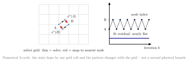
vaft.diagram.grid_induced_two_cycle()A numerical 2-cycle: the discrete state hops between two adjacent grid nodes.
vaft.diagram.grid_induced_two_cycle(*, labels=True)Show source vaft/diagram/_iteration_dynamics.py, lines 262–328
def grid_induced_two_cycle(*, labels: bool = True) -> Diagram:
r"""A numerical 2-cycle: the discrete state hops between two adjacent grid nodes.
The solve depends on the discrete state it starts from -- a magnetic
axis located on a grid node, say. Solved from node A, the continuous
optimum $x^*(A)$ lands nearer B, so the state snaps to B; solved from B,
$x^*(B)$ lands nearer A, and the state snaps back. The node-to-node map
has no fixed point, so a convergence test on the state is never met,
while the fit and the continuous state hardly change. What separates
this from a physical branch switch: the hop is exactly one grid cell,
and the pattern changes when the grid is refined; the flat fit residual
on the right is the secondary cue (two symmetric physical branches can
also fit equally well).
"""
labels = _check_labels(labels)
xs, ys = np.arange(_NX) * _DX, np.arange(_NY) * _DX
items: List = []
for x in xs:
items.append(Polyline.of([(x, ys[0]), (x, ys[-1])], "mesh", role="grid"))
for y in ys:
items.append(Polyline.of([(xs[0], y), (xs[-1], y)], "mesh", role="grid"))
a, b = (2.0, 2.0), (3.0, 2.0)
# the optimum each re-solve finds, just past the midpoint towards the other node
from_a, from_b = (2.62, 2.45), (2.38, 1.55)
items += [Marker(a, "o", "opoint", role="cell_A"), Marker(b, "o", "opoint", role="cell_B"),
Marker(from_a, "x", "xpoint", role="optimum_from_A"),
Marker(from_b, "x", "xpoint", role="optimum_from_B"),
# solve (thin), then snap to the nearest node (red)
Arrow((a[0] + 0.08, a[1] + 0.06), (from_a[0] - 0.08, from_a[1] - 0.04), "connector", role="solve"),
Arrow((from_a[0] + 0.06, from_a[1] - 0.08), (b[0] - 0.05, b[1] + 0.1), "drift", role="hop"),
Arrow((b[0] - 0.08, b[1] - 0.06), (from_b[0] + 0.08, from_b[1] + 0.04), "connector", role="solve"),
Arrow((from_b[0] - 0.06, from_b[1] + 0.08), (a[0] + 0.05, a[1] - 0.1), "drift", role="hop")]
# right: discrete index and fit residual against iteration
ox, w, h = xs[-1] + 2.1, 4.0, ys[-1]
k = np.arange(12)
levels = {"A": 0.38 * h, "B": 0.62 * h}
index = np.where(k % 2 == 0, levels["A"], levels["B"])
residual = np.full(k.shape, 0.15 * h)
kx = ox + k * w / 11
items += [Arrow((ox, 0.0), (ox + w + 0.3, 0.0), "chart axis", role="axes"),
Arrow((ox, 0.0), (ox, h + 0.3), "chart axis", role="axes"),
Polyline.of(np.stack([kx, index], axis=-1), "connector line", role="index"),
Polyline.of(np.stack([kx, residual], axis=-1), "boundary", role="residual")]
items += [Marker((float(x), float(y)), "o", "xpoint", role="index") for x, y in zip(kx, index)]
for name, y in levels.items():
items.append(Polyline.of([(ox, y), (ox - 0.12, y)], "tick", role="ticks"))
if labels:
items += [Label((a[0] - 0.1, a[1] - 0.1), "A", "small label", anchor="north east", role="cell_A"),
Label((b[0] + 0.1, b[1] + 0.1), "B", "small label", anchor="south west", role="cell_B"),
Label((from_a[0] + 0.1, from_a[1] + 0.05), "$x^*(A)$", "small label", anchor="south west",
role="optimum_from_A"),
Label((from_b[0] - 0.1, from_b[1] - 0.05), "$x^*(B)$", "small label", anchor="north east",
role="optimum_from_B"),
Label((xs[-1] / 2, -0.35), "solver grid: thin = solve, red = snap to nearest node", "small label",
anchor="north", role="grid"),
Label((ox + w + 0.3, -0.1), "iteration $k$", "small label", anchor="north", role="axes"),
Label((ox + w, max(levels.values()) + 0.3), "node index", "small label", anchor="south east",
role="index"),
Label((ox + w, residual[-1] + 0.15), "fit residual: nearly flat", "small label",
anchor="south east", role="residual"),
Label((ox / 2 + w / 2, -1.1), "Numerical 2-cycle: the state hops by one grid cell and the pattern "
"changes with the grid -- not a second physical branch", "note", anchor="north",
role="note")]
items += [Label((ox - 0.18, y), name, "ticklabel", anchor="east", role="ticks") for name, y in levels.items()]
return Diagram("grid_induced_two_cycle", Scene(tuple(items)),
model={"cell_A": a, "cell_B": b, "optimum_from_A": from_a, "optimum_from_B": from_b,
"grid_spacing": _DX})Formats .svg .tex .pdf the SVG above is committed; build the others locally
import vaft.diagram
d = vaft.diagram.grid_induced_two_cycle()
d.tikz # the TikZ document as text
d.save("grid_induced_two_cycle.svg") # rendered vector image, the canonical artifact; needs latex, dvisvgm
d.save("grid_induced_two_cycle.tex") # the complete TikZ document, the text source
d.save("grid_induced_two_cycle.pdf") # vector PDF; needs pdflatexbranch_selection
1 asset
source
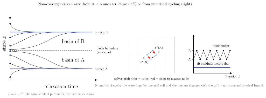
vaft.diagram.branch_selection()Physical branch selection beside numerical cycling: the two causes of non-convergence side by side.
vaft.diagram.branch_selection(*, labels=True)Show source vaft/diagram/_iteration_dynamics.py, lines 331–347
def branch_selection(*, labels: bool = True) -> Diagram:
r"""Physical branch selection beside numerical cycling: the two causes of non-convergence side by side.
``basin_of_attraction`` (two physical solutions, the start decides) and
``grid_induced_two_cycle`` (one solution, a discrete state that cannot
settle) composed under one caption. No new physics: the two panels are
those diagrams unchanged.
"""
labels = _check_labels(labels)
left = basin_of_attraction(labels=labels).scene
right = grid_induced_two_cycle(labels=labels).scene.transformed(offset=(13.0, 0.75))
items = list(left.items) + list(right.items)
if labels:
items.append(Label((11.5, 8.0), "Non-convergence can arise from true branch structure (left) or from "
"numerical cycling (right)", "label", anchor="south", role="caption"))
return Diagram("branch_selection", Scene(tuple(items)),
model={"panels": ("basin_of_attraction", "grid_induced_two_cycle")})Formats .svg .tex .pdf the SVG above is committed; build the others locally
import vaft.diagram
d = vaft.diagram.branch_selection()
d.tikz # the TikZ document as text
d.save("branch_selection.svg") # rendered vector image, the canonical artifact; needs latex, dvisvgm
d.save("branch_selection.tex") # the complete TikZ document, the text source
d.save("branch_selection.pdf") # vector PDF; needs pdflatexCold-plasma waves from their equations: O and X modes, the CMA diagram and a profile’s cutoffs
Module vaft.diagram._cold_plasma_waves
o_mode_cutoff
1 asset
source
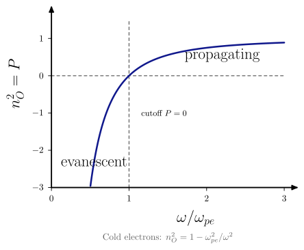
vaft.diagram.o_mode_cutoff()O-mode refractive index against frequency: propagation above $\omega_{pe}$, evanescence below.
vaft.diagram.o_mode_cutoff(*, labels=True)Show source vaft/diagram/_cold_plasma_waves.py, lines 93–120
def o_mode_cutoff(*, labels: bool = True) -> Diagram:
r"""O-mode refractive index against frequency: propagation above $\omega_{pe}$, evanescence below.
$n_O^2 = P = 1 - \omega_{pe}^2/\omega^2$ from ``stix_parameters``; the
cutoff $P = 0$ is located by bracketing the formula and lands on
$\omega = \omega_{pe}$. Independent of $B$.
"""
labels = _check_labels(labels)
ratio = np.linspace(0.35, 3.0, 400)
omega = ratio * _W_REF
P = _electron_stix(omega, _N_REF, 0.0).P
cutoff = _bisect(lambda r: _electron_stix(r * _W_REF, _N_REF, 0.0).P, 0.5, 2.0)
chart = Chart(x_range=(0.0, 3.0), y_range=(-3.0, 1.5))
chart.curves["n2_O"] = np.stack([ratio, P], axis=-1)[P >= -3.0]
chart.curves["zero"] = np.array([[0.0, 0.0], [3.0, 0.0]])
chart.curves["cutoff"] = np.array([[cutoff, -3.0], [cutoff, 1.5]])
chart.points["cutoff"] = (cutoff, 0.0)
chart.labels.update({"evanescent": (0.55, -2.3), "propagating": (2.2, 0.55), "cutoff": (cutoff + 0.45, -1.0)})
chart.parameters.update({"cutoff_omega_over_omega_pe": cutoff})
scene = render_chart(
chart, x_label="$\\omega/\\omega_{pe}$", y_label="$n_O^2 = P$",
curve_styles={"zero": "approx", "cutoff": "approx", "n2_O": "boundary"},
region_text={"evanescent": "evanescent", "propagating": "propagating",
"cutoff": "\\small cutoff $P = 0$"} if labels else {},
x_ticks=[0.0, 1.0, 2.0, 3.0], y_ticks=[-3.0, -2.0, -1.0, 0.0, 1.0],
note="Cold electrons: $n_O^2 = 1 - \\omega_{pe}^2/\\omega^2$" if labels else "",
)
return Diagram("o_mode_cutoff", scene, model=chart)Formats .svg .tex .pdf the SVG above is committed; build the others locally
import vaft.diagram
d = vaft.diagram.o_mode_cutoff()
d.tikz # the TikZ document as text
d.save("o_mode_cutoff.svg") # rendered vector image, the canonical artifact; needs latex, dvisvgm
d.save("o_mode_cutoff.tex") # the complete TikZ document, the text source
d.save("o_mode_cutoff.pdf") # vector PDF; needs pdflatexFormula functions referenced:
waves.stix_parameters
x_mode_dispersion
1 asset
source
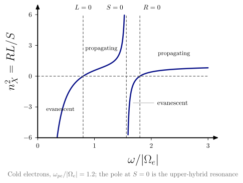
vaft.diagram.x_mode_dispersion()X-mode refractive index against frequency: two cutoffs, the upper-hybrid resonance and two gaps.
vaft.diagram.x_mode_dispersion(*, omega_pe_over_omega_ce=1.2, labels=True)Show source vaft/diagram/_cold_plasma_waves.py, lines 123–186
def x_mode_dispersion(*, omega_pe_over_omega_ce: float = 1.2, labels: bool = True) -> Diagram:
r"""X-mode refractive index against frequency: two cutoffs, the upper-hybrid resonance and two gaps.
$n_X^2 = RL/S$ from ``perpendicular_refractive_index_squared``, for a
cold electron plasma with $\omega_{pe}/|\Omega_e|$ =
``omega_pe_over_omega_ce``. Located from the formula by bracketing: the
$L$ cutoff $\omega_L$, the upper-hybrid resonance $S = 0$ at
$\omega_{UH}$, and the $R$ cutoff $\omega_R$. The X mode is evanescent
below $\omega_L$, propagates
between $\omega_L$ and $\omega_{UH}$, is evanescent between
$\omega_{UH}$ and $\omega_R$, and propagates above $\omega_R$. Poles are
masked, not drawn through.
"""
labels = _check_labels(labels)
if not omega_pe_over_omega_ce > 0.0:
raise ValueError("omega_pe_over_omega_ce must be positive")
n_e = _N_REF * omega_pe_over_omega_ce**2 # omega_pe in units of the reference, |Omega_e| = reference
B = _field_for_Y(1.0, _W_REF)
stix = lambda r: _electron_stix(r * _W_REF, n_e, B)
w_uh_guess = np.sqrt(1.0 + omega_pe_over_omega_ce**2)
omega_L = _bisect(lambda r: stix(r).L, 1e-3, w_uh_guess - 1e-6)
omega_UH = _bisect(lambda r: stix(r).S, 1.0 + 1e-9, 3.5 * w_uh_guess)
omega_R = _bisect(lambda r: stix(r).R, 1.0 + 1e-9, 3.5 * w_uh_guess)
x_max = float(np.ceil(1.4 * omega_R * 2.0) / 2.0)
ratio = np.linspace(0.05, x_max, 1400)
s = _electron_stix(ratio * _W_REF, n_e, B)
_, n2_X = perpendicular_refractive_index_squared(s.R, s.L, s.P)
limit = 6.0
chart = Chart(x_range=(0.0, x_max), y_range=(-limit, limit))
for i, run in enumerate(_clip_runs(ratio, np.asarray(n2_X), limit)):
chart.curves[f"n2_X {i}"] = run
chart.curves["zero"] = np.array([[0.0, 0.0], [x_max, 0.0]])
for name, value in (("omega_L", omega_L), ("omega_UH", omega_UH), ("omega_R", omega_R)):
chart.curves[name] = np.array([[value, -limit], [value, limit]])
chart.points[name] = (value, 0.0)
chart.labels.update({"gap1": (omega_L / 2, -3.2), "prop": (0.5 * (omega_R + x_max), 2.2),
"prop_low": (0.5 * (omega_L + omega_UH) - 0.06, 2.7)})
chart.parameters.update({"omega_pe_over_omega_ce": omega_pe_over_omega_ce, "omega_L": omega_L,
"omega_UH": omega_UH, "omega_R": omega_R})
styles: Dict[str, str] = {name: "boundary" for name in chart.curves if name.startswith("n2_X")}
styles.update({"zero": "approx", "omega_L": "approx", "omega_UH": "approx", "omega_R": "approx"})
scene = render_chart(
chart, x_label="$\\omega/|\\Omega_e|$", y_label="$n_X^2 = RL/S$", curve_styles=styles,
region_text={"gap1": "\\small evanescent", "prop": "\\small propagating",
"prop_low": "\\small propagating"} if labels else {},
x_ticks=[float(v) for v in range(int(x_max) + 1)], y_ticks=[-6.0, -3.0, 0.0, 3.0, 6.0],
note=(f"Cold electrons, $\\omega_{{pe}}/|\\Omega_e| = {omega_pe_over_omega_ce:g}$; "
"the pole at $S = 0$ is the upper-hybrid resonance" if labels else ""),
)
items = list(scene.items)
if labels:
cm = chart.to_cm
top = float(cm(np.array([0.0, limit]))[1]) + 0.15
items += [Label((float(cm(np.array([omega_L, 0.0]))[0]), top), "$L = 0$", "small label", anchor="south",
role="omega_L"),
Label((float(cm(np.array([omega_UH, 0.0]))[0]) - 0.05, top), "$S = 0$", "small label",
anchor="south east", role="omega_UH"),
Label((float(cm(np.array([omega_R, 0.0]))[0]) + 0.05, top), "$R = 0$", "small label",
anchor="south west", role="omega_R")]
gap = cm(np.array([0.5 * (omega_UH + omega_R), -2.6]))
items += [Polyline.of([tuple(gap), (float(gap[0]) + 1.1, float(gap[1]))], "leader line", role="gap2"),
Label((float(gap[0]) + 1.15, float(gap[1])), "evanescent", "small label", anchor="west",
role="gap2")]
return Diagram("x_mode_dispersion", Scene(tuple(items)), model=chart)Formats .svg .tex .pdf the SVG above is committed; build the others locally
import vaft.diagram
d = vaft.diagram.x_mode_dispersion()
d.tikz # the TikZ document as text
d.save("x_mode_dispersion.svg") # rendered vector image, the canonical artifact; needs latex, dvisvgm
d.save("x_mode_dispersion.tex") # the complete TikZ document, the text source
d.save("x_mode_dispersion.pdf") # vector PDF; needs pdflatexFormula functions referenced:
waves.perpendicular_refractive_index_squared, waves.stix_parameters
cma_diagram
1 asset
source
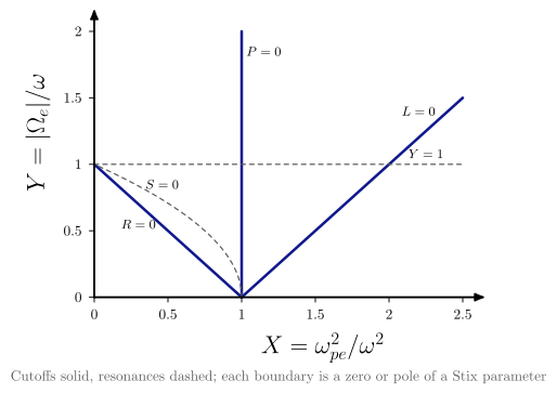
vaft.diagram.cma_diagram()The Clemmow–Mullaly–Allis diagram of a cold electron plasma.
vaft.diagram.cma_diagram(*, labels=True)Show source vaft/diagram/_cold_plasma_waves.py, lines 204–234
def cma_diagram(*, labels: bool = True) -> Diagram:
r"""The Clemmow--Mullaly--Allis diagram of a cold electron plasma.
Horizontal $X = \omega_{pe}^2/\omega^2$, vertical $Y = |\Omega_e|/\omega$
(``cma_coordinates``). The cutoffs $P = 0$ (O mode), $R = 0$ and $L = 0$
(X mode), the upper-hybrid resonance $S = 0$ and the cyclotron resonance
$Y = 1$ (a pole of $R$), each found as the zero of the Stix parameter
from ``stix_parameters`` at every $Y$. Ions immobile, so the ion
resonances and the lower hybrid lie off this chart.
"""
labels = _check_labels(labels)
Y = np.linspace(0.0, 2.0, 201)
bounds = cma_boundaries(Y)
chart = Chart(x_range=(0.0, 2.5), y_range=(0.0, 2.0))
for name in ("P", "R", "L", "S"):
ok = np.isfinite(bounds[name])
chart.curves[f"{name}=0"] = np.stack([bounds[name][ok], Y[ok]], axis=-1)
chart.curves["Y=1"] = np.array([[0.0, 1.0], [2.5, 1.0]])
chart.labels.update({"P": (1.15, 1.85), "R": (0.3, 0.55), "L": (2.2, 1.4), "S": (0.46, 0.85),
"Y": (2.25, 1.08)})
chart.parameters.update({"electrons_only": 1.0})
styles = {"P=0": "boundary", "R=0": "boundary", "L=0": "boundary", "S=0": "approx", "Y=1": "approx"}
scene = render_chart(
chart, x_label="$X = \\omega_{pe}^2/\\omega^2$", y_label="$Y = |\\Omega_e|/\\omega$", curve_styles=styles,
region_text={"P": "\\small $P = 0$", "R": "\\small $R = 0$", "L": "\\small $L = 0$",
"S": "\\small $S = 0$", "Y": "\\small $Y = 1$"} if labels else {},
x_ticks=[0.0, 0.5, 1.0, 1.5, 2.0, 2.5], y_ticks=[0.0, 0.5, 1.0, 1.5, 2.0],
note=("Cutoffs solid, resonances dashed; each boundary is a zero or pole of a Stix parameter"
if labels else ""),
)
return Diagram("cma_diagram", scene, model=chart)Formats .svg .tex .pdf the SVG above is committed; build the others locally
import vaft.diagram
d = vaft.diagram.cma_diagram()
d.tikz # the TikZ document as text
d.save("cma_diagram.svg") # rendered vector image, the canonical artifact; needs latex, dvisvgm
d.save("cma_diagram.tex") # the complete TikZ document, the text source
d.save("cma_diagram.pdf") # vector PDF; needs pdflatexFormula functions referenced:
waves.stix_parameters
profile_propagation
2 assets
source
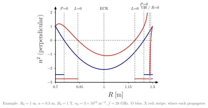
vaft.diagram.profile_propagation()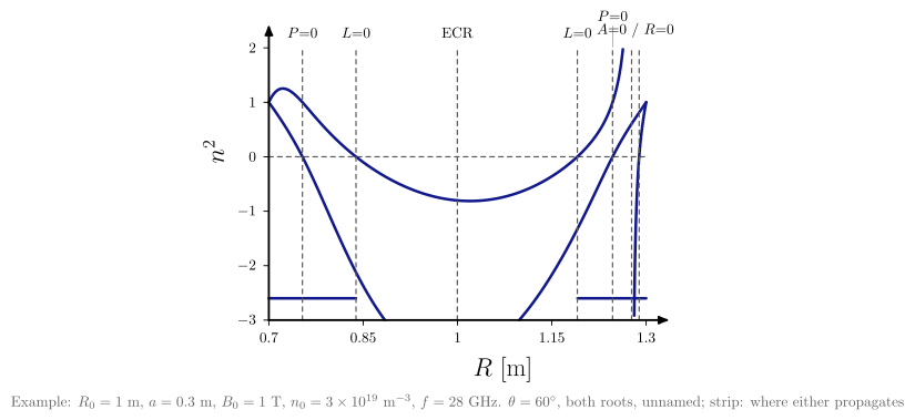
vaft.diagram.profile_propagation(theta=1.0471975511965976)O- and X-mode $n^2$ along the midplane of an example tokamak, with its cutoff and resonance layers.
vaft.diagram.profile_propagation(*, theta=None, labels=True)Formats .svg .tex .pdf the SVG above is committed; build the others locally
import vaft.diagram
d = vaft.diagram.profile_propagation()
d.tikz # the TikZ document as text
d.save("profile_propagation.svg") # rendered vector image, the canonical artifact; needs latex, dvisvgm
d.save("profile_propagation.tex") # the complete TikZ document, the text source
d.save("profile_propagation.pdf") # vector PDF; needs pdflatexFormula functions referenced:
waves.cold_plasma_refractive_index_squared, waves.perpendicular_refractive_index_squared, waves.propagation_regime, waves.stix_parameters
wave_dispersion_omega_k
2 assets
source
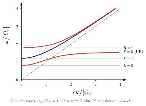
vaft.diagram.wave_dispersion_omega_k()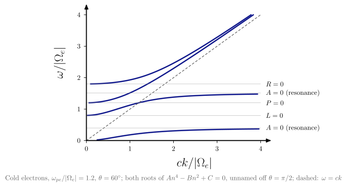
vaft.diagram.wave_dispersion_omega_k(theta=1.0471975511965976)The cold electron plasma in the $\omega$-$k$ plane: where each branch exists and where it ends.
vaft.diagram.wave_dispersion_omega_k(*, omega_pe_over_omega_ce=1.2, theta=1.5707963267948966, labels=True)Show source vaft/diagram/_cold_plasma_waves.py, lines 423–490
def wave_dispersion_omega_k(*, omega_pe_over_omega_ce: float = 1.2, theta: float = 0.5 * np.pi,
labels: bool = True) -> Diagram:
r"""The cold electron plasma in the $\omega$-$k$ plane: where each branch exists and where it ends.
For each frequency the refractive index from the Stix parameters gives
$k = n\omega/c$ wherever $n^2 > 0$; the branches start at $k = 0$ on their
cutoffs ($P$, $R$ or $L = 0$) -- except the oblique whistler, which leaves
the origin -- and run to $k \to \infty$ at a resonance
($S = 0$, the upper hybrid, at $\theta = \pi/2$), approaching the light
line $\omega = ck$ from above at high frequency. ``theta = pi/2`` names
the branches O and X (``perpendicular_refractive_index_squared``);
another angle draws both roots of ``cold_plasma_refractive_index_squared``
in one colour, since its algebraic $\pm$ branches swap at the cyclotron
layer, and marks the resonances $A = S\sin^2\theta + P\cos^2\theta = 0$.
Axes in units of $|\Omega_e|$.
"""
labels = _check_labels(labels)
theta = _check_theta(theta)
omega_pe_over_omega_ce = _number(omega_pe_over_omega_ce, "omega_pe_over_omega_ce")
if not 0.0 < omega_pe_over_omega_ce <= 3.0:
raise ValueError(f"omega_pe_over_omega_ce must be in (0, 3] to keep the cutoffs on the chart, "
f"not {omega_pe_over_omega_ce!r}")
n_e = _N_REF * omega_pe_over_omega_ce**2
B = _field_for_Y(1.0, _W_REF)
w = np.linspace(0.02, 4.0, 3000)
s = _electron_stix(w * _W_REF, n_e, B)
k_max = 4.0
chart = Chart(x_range=(0.0, k_max), y_range=(0.0, 4.0))
for name, n2 in _modes(s, theta).items():
with np.errstate(invalid="ignore"):
k = np.where(np.isfinite(n2) & (n2 > 0), np.sqrt(np.clip(n2, 0, None)) * w, np.nan)
for i, run in enumerate(_clip_runs(w, k, k_max)):
chart.curves[f"{name} {i}"] = run[:, ::-1] # (k, omega)
chart.curves["light"] = np.array([[0.0, 0.0], [4.0, 4.0]])
stix = lambda r: _electron_stix(r * _W_REF, n_e, B)
w_uh = np.sqrt(1.0 + omega_pe_over_omega_ce**2)
layers = {"P": _bisect(lambda r: stix(r).P, 1e-3, 10.0),
"L": _bisect(lambda r: stix(r).L, 1e-3, w_uh - 1e-6),
"R": _bisect(lambda r: stix(r).R, 1.0 + 1e-9, 3.5 * w_uh)}
if np.isclose(theta, 0.5 * np.pi):
layers["S"] = _bisect(lambda r: stix(r).S, 1.0 + 1e-9, 3.5 * w_uh)
else:
layers.update({("A" if i == 0 else f"A{i + 1}"): r for i, r in enumerate(_resonance_cone(np.linspace(0.02, 4.0, 801), stix, theta))})
for name, value in layers.items():
if chart.y_range[0] < value < chart.y_range[1]:
chart.curves[f"layer {name}"] = np.array([[0.0, value], [k_max, value]])
chart.parameters.update({"omega_pe_over_omega_ce": omega_pe_over_omega_ce, "theta": theta,
**{f"omega_{k}": v for k, v in layers.items()}})
styles = {n: _BRANCH_STYLE[n.split(" ")[0]] for n in chart.curves if n.split(" ")[0] in _BRANCH_STYLE}
styles.update({"light": "approx"})
styles.update({n: "mesh" for n in chart.curves if n.startswith("layer")})
scene = render_chart(
chart, x_label="$ck/|\\Omega_e|$", y_label="$\\omega/|\\Omega_e|$", curve_styles=styles, region_text={},
x_ticks=[0.0, 1.0, 2.0, 3.0, 4.0], y_ticks=[0.0, 1.0, 2.0, 3.0, 4.0],
note=(f"Cold electrons, $\\omega_{{pe}}/|\\Omega_e| = {omega_pe_over_omega_ce:g}$, ${_theta_text(theta)}$; "
f"{_branch_note(theta)}; dashed: $\\omega = ck$" if labels else ""),
)
items = list(scene.items)
if labels:
text = {"P": "$P = 0$", "L": "$L = 0$", "R": "$R = 0$", "S": "$S = 0$ (UH)", "A": "$A = 0$ (resonance)",
"A2": "$A = 0$ (resonance)"}
x = float(chart.to_cm(np.array([k_max, 0.0]))[0]) + 0.15
for name, value in sorted(layers.items(), key=lambda kv: kv[1]):
if not chart.y_range[0] < value < chart.y_range[1]:
continue
y = float(chart.to_cm(np.array([0.0, value]))[1])
items.append(Label((x, y), text[name], "small label", anchor="west", role=f"layer {name}"))
return Diagram("wave_dispersion_omega_k", Scene(tuple(items)), model=chart)Formats .svg .tex .pdf the SVG above is committed; build the others locally
import vaft.diagram
d = vaft.diagram.wave_dispersion_omega_k()
d.tikz # the TikZ document as text
d.save("wave_dispersion_omega_k.svg") # rendered vector image, the canonical artifact; needs latex, dvisvgm
d.save("wave_dispersion_omega_k.tex") # the complete TikZ document, the text source
d.save("wave_dispersion_omega_k.pdf") # vector PDF; needs pdflatexFormula functions referenced:
waves.cold_plasma_refractive_index_squared, waves.perpendicular_refractive_index_squared, waves.stix_parameters
refractive_index_vs_X
2 assets
source
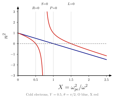
vaft.diagram.refractive_index_vs_X()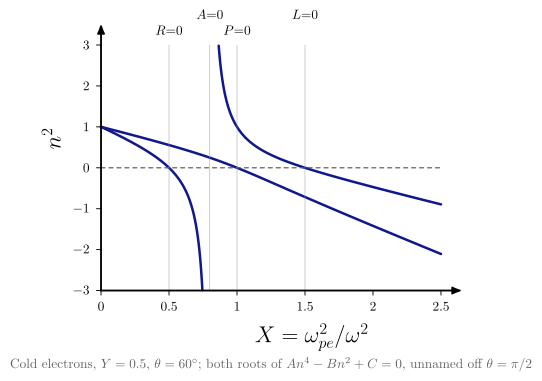
vaft.diagram.refractive_index_vs_X(theta=1.0471975511965976)$n^2$ against $X = \omega_{pe}^2/\omega^2$ at fixed $Y$: rising density at one frequency and field.
vaft.diagram.refractive_index_vs_X(*, Y=0.5, theta=1.5707963267948966, labels=True)Show source vaft/diagram/_cold_plasma_waves.py, lines 539–570
def refractive_index_vs_X(*, Y: float = 0.5, theta: float = 0.5 * np.pi, labels: bool = True) -> Diagram:
r"""$n^2$ against $X = \omega_{pe}^2/\omega^2$ at fixed $Y$: rising density at one frequency and field.
The cutoffs are the zeros of the Stix parameters along $X$ -- $P = 0$ at
$X = 1$, $R = 0$ at $X = 1 - Y$, $L = 0$ at $X = 1 + Y$ -- and at
$\theta = \pi/2$ the upper-hybrid resonance $S = 0$ at $X = 1 - Y^2$,
all located by bracketing ``stix_parameters`` rather than from these
closed forms. Branches as in ``wave_dispersion_omega_k``.
"""
labels = _check_labels(labels)
theta = _check_theta(theta)
Y = _number(Y, "Y")
if not 0.0 < Y < 1.0:
raise ValueError(f"Y must be between 0 and 1 (below the cyclotron resonance), not {Y!r}")
X = np.linspace(0.0, 2.5, 2000)
B = _field_for_Y(Y, _W_REF)
s = _electron_stix(_W_REF, _density_for_X(X, _W_REF), B)
at = lambda name: (lambda x: getattr(_electron_stix(_W_REF, _density_for_X(x, _W_REF), B), name))
layers = {"P": _bisect(at("P"), 0.5, 2.0), "R": _bisect(at("R"), 1e-6, 1.0),
"L": _bisect(at("L"), 1.0, 2.5)}
if np.isclose(theta, 0.5 * np.pi):
layers["S"] = _bisect(at("S"), 1e-6, 1.0 - 1e-9)
else:
layers.update({("A" if i == 0 else f"A{i + 1}"): r for i, r in enumerate(_resonance_cone(
np.linspace(1e-6, 2.5, 501), lambda x: _electron_stix(_W_REF, _density_for_X(x, _W_REF), B), theta))})
chart, styles, note = _index_chart("X", X, s, theta, layers, f"Cold electrons, $Y = {Y:g}$")
chart.parameters.update({"Y": Y, "theta": theta, **{f"X_{k}": v for k, v in layers.items()}})
scene = render_chart(chart, x_label="$X = \\omega_{pe}^2/\\omega^2$", y_label="$n^2$", curve_styles=styles,
region_text={}, x_ticks=[0.0, 0.5, 1.0, 1.5, 2.0, 2.5],
y_ticks=[-3.0, -2.0, -1.0, 0.0, 1.0, 2.0, 3.0], note=note if labels else "")
items = list(scene.items) + (_layer_labels(chart, layers, _LAYER_TEXT) if labels else [])
return Diagram("refractive_index_vs_X", Scene(tuple(items)), model=chart)Formats .svg .tex .pdf the SVG above is committed; build the others locally
import vaft.diagram
d = vaft.diagram.refractive_index_vs_X()
d.tikz # the TikZ document as text
d.save("refractive_index_vs_X.svg") # rendered vector image, the canonical artifact; needs latex, dvisvgm
d.save("refractive_index_vs_X.tex") # the complete TikZ document, the text source
d.save("refractive_index_vs_X.pdf") # vector PDF; needs pdflatexFormula functions referenced:
waves.cold_plasma_refractive_index_squared, waves.perpendicular_refractive_index_squared, waves.stix_parameters
refractive_index_vs_Y
2 assets
source
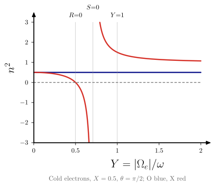
vaft.diagram.refractive_index_vs_Y()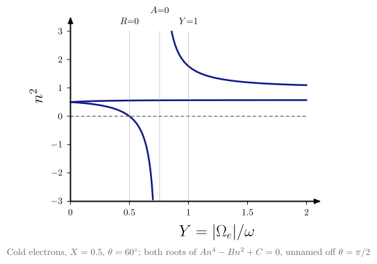
vaft.diagram.refractive_index_vs_Y(theta=1.0471975511965976)| $n^2$ against $Y = | \Omega_e | /\omega$ at fixed $X$: rising field at one frequency and density. |
vaft.diagram.refractive_index_vs_Y(*, X=0.5, theta=1.5707963267948966, labels=True)Show source vaft/diagram/_cold_plasma_waves.py, lines 573–603
def refractive_index_vs_Y(*, X: float = 0.5, theta: float = 0.5 * np.pi, labels: bool = True) -> Diagram:
r"""$n^2$ against $Y = |\Omega_e|/\omega$ at fixed $X$: rising field at one frequency and density.
At $\theta = \pi/2$ the O branch ($n^2 = P = 1 - X$) does not depend on $Y$; the other
branch has the $R = 0$ cutoff at $Y = 1 - X$ and, at $\theta = \pi/2$,
the upper-hybrid resonance $S = 0$ at $Y = \sqrt{1 - X}$; $Y = 1$ is the
electron cyclotron resonance, where $R$ has its pole. Located by
bracketing ``stix_parameters``. Branches as in ``wave_dispersion_omega_k``.
"""
labels = _check_labels(labels)
theta = _check_theta(theta)
X = _number(X, "X")
if not 0.0 < X < 1.0:
raise ValueError(f"X must be between 0 and 1 (above the O cutoff), not {X!r}")
Yv = np.linspace(0.0, 2.0, 2001)[1:]
n_e = _density_for_X(X, _W_REF)
s = _electron_stix(_W_REF, n_e, _field_for_Y(Yv, _W_REF))
at = lambda name: (lambda y: getattr(_electron_stix(_W_REF, n_e, _field_for_Y(y, _W_REF)), name))
layers = {"R": _bisect(at("R"), 1e-6, 1.0 - 1e-9), "ECR": 1.0}
if np.isclose(theta, 0.5 * np.pi):
layers["S"] = _bisect(at("S"), 1e-6, 1.0 - 1e-9)
else:
layers.update({("A" if i == 0 else f"A{i + 1}"): r for i, r in enumerate(_resonance_cone(
np.linspace(1e-3, 2.0, 801), lambda y: _electron_stix(_W_REF, n_e, _field_for_Y(y, _W_REF)), theta))})
chart, styles, note = _index_chart("Y", Yv, s, theta, layers, f"Cold electrons, $X = {X:g}$")
chart.parameters.update({"X": X, "theta": theta, **{f"Y_{k}": v for k, v in layers.items()}})
scene = render_chart(chart, x_label="$Y = |\\Omega_e|/\\omega$", y_label="$n^2$", curve_styles=styles,
region_text={}, x_ticks=[0.0, 0.5, 1.0, 1.5, 2.0],
y_ticks=[-3.0, -2.0, -1.0, 0.0, 1.0, 2.0, 3.0], note=note if labels else "")
items = list(scene.items) + (_layer_labels(chart, layers, _LAYER_TEXT) if labels else [])
return Diagram("refractive_index_vs_Y", Scene(tuple(items)), model=chart)Formats .svg .tex .pdf the SVG above is committed; build the others locally
import vaft.diagram
d = vaft.diagram.refractive_index_vs_Y()
d.tikz # the TikZ document as text
d.save("refractive_index_vs_Y.svg") # rendered vector image, the canonical artifact; needs latex, dvisvgm
d.save("refractive_index_vs_Y.tex") # the complete TikZ document, the text source
d.save("refractive_index_vs_Y.pdf") # vector PDF; needs pdflatexFormula functions referenced:
waves.cold_plasma_refractive_index_squared, waves.perpendicular_refractive_index_squared, waves.stix_parameters
Collisionality regimes: axisymmetric neoclassical and non-axisymmetric NTV
Module vaft.diagram._transport_regimes
neoclassical_collisionality
1 asset
source
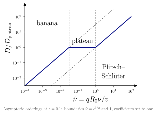
vaft.diagram.neoclassical_collisionality()Banana, plateau and Pfirsch–Schl"uter: the axisymmetric neoclassical regimes.
vaft.diagram.neoclassical_collisionality(*, epsilon=0.1, labels=True)Show source vaft/diagram/_transport_regimes.py, lines 41–88
def neoclassical_collisionality(*, epsilon: float = 0.1, labels: bool = True) -> Diagram:
r"""Banana, plateau and Pfirsch--Schl\"uter: the axisymmetric neoclassical regimes.
The horizontal axis is $\hat\nu = qR_0\nu/v$ (``collisions_per_transit``),
not a $\nu_*$ convention; the boundaries $\hat\nu = \epsilon^{3/2}$ and
$\hat\nu = 1$ come from ``neoclassical_regime_boundaries``. The vertical
axis is the diffusivity in units of the plateau value, with the three
textbook asymptotes $\hat\nu/\epsilon^{3/2}$, $1$ and $\hat\nu$ (order-unity
coefficients set to one), which meet exactly at those boundaries. Lower
$\epsilon$ widens the plateau.
"""
labels = _check_labels(labels)
if not 0.0 < epsilon < 1.0:
raise ValueError(f"epsilon must lie in (0, 1), not {epsilon!r}")
banana_plateau, plateau_ps = neoclassical_regime_boundaries(epsilon)
xb, xp = float(np.log10(banana_plateau)), float(np.log10(plateau_ps))
x = np.linspace(-4.0, 2.0, 301)
nu = 10.0 ** x
banana, plateau, ps = nu / banana_plateau, np.ones_like(nu), nu / plateau_ps
total = np.minimum(banana, np.maximum(plateau, ps))
chart = Chart(x_range=(-4.0, 2.0), y_range=(-2.5, 2.5))
chart.curves.update({
"diffusivity": np.stack([x, np.log10(total)], axis=-1),
"banana_asymptote": np.stack([x, np.log10(banana)], axis=-1),
"pfirsch_schlueter_asymptote": np.stack([x, np.log10(ps)], axis=-1),
"banana_plateau": np.array([[xb, -2.5], [xb, 2.5]]),
"plateau_pfirsch_schlueter": np.array([[xp, -2.5], [xp, 2.5]]),
})
chart.labels.update({"banana": ((-4.0 + xb) / 2, 1.6), "plateau": ((xb + xp) / 2, 0.4),
"pfirsch_schlueter": ((xp + 2.0) / 2, -1.6)})
chart.parameters.update({"epsilon": epsilon, "banana_plateau": banana_plateau,
"plateau_pfirsch_schlueter": plateau_ps})
x_ticks, x_text = _decades(-4, 2)
y_ticks, y_text = _decades(-2, 2)
scene = render_chart(
chart,
x_label="$\\hat\\nu = qR_0\\nu/v$",
y_label="$D/D_\\mathrm{plateau}$",
curve_styles={"banana_asymptote": "approx", "pfirsch_schlueter_asymptote": "approx",
"banana_plateau": "approx", "plateau_pfirsch_schlueter": "approx", "diffusivity": "boundary"},
region_text={"banana": "banana", "plateau": "plateau",
"pfirsch_schlueter": "\\begin{tabular}{c}Pfirsch--\\\\Schl\\\"uter\\end{tabular}"}
if labels else {},
x_ticks=x_ticks, x_tick_text=x_text, y_ticks=y_ticks, y_tick_text=y_text,
note=(f"Asymptotic orderings at $\\epsilon = {epsilon:g}$: boundaries $\\hat\\nu = \\epsilon^{{3/2}}$ "
"and 1, coefficients set to one" if labels else ""),
)
return Diagram("neoclassical_collisionality", scene, model=chart)Formats .svg .tex .pdf the SVG above is committed; build the others locally
import vaft.diagram
d = vaft.diagram.neoclassical_collisionality()
d.tikz # the TikZ document as text
d.save("neoclassical_collisionality.svg") # rendered vector image, the canonical artifact; needs latex, dvisvgm
d.save("neoclassical_collisionality.tex") # the complete TikZ document, the text source
d.save("neoclassical_collisionality.pdf") # vector PDF; needs pdflatexFormula functions referenced:
neoclassical.neoclassical_regime_boundaries
ntv_collisionality
1 asset
source
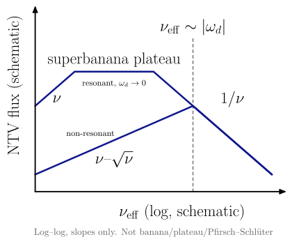
vaft.diagram.ntv_collisionality()Shaing’s NTV regimes: the non-resonant and resonant branches of the flux against collisionality.
vaft.diagram.ntv_collisionality(*, labels=True)Show source vaft/diagram/_transport_regimes.py, lines 95–136
def ntv_collisionality(*, labels: bool = True) -> Diagram:
r"""Shaing's NTV regimes: the non-resonant and resonant branches of the flux against collisionality.
Schematic in both axes: only the slopes are physics -- the asymptotic
exponents of ``NTV_EXPONENTS`` -- and the breakpoints are placed for
legibility. Non-resonant ($\omega_d$ bounded away from zero): $1/\nu$
while $\nu_\mathrm{eff}$ exceeds the precession, then the
$\nu$--$\sqrt\nu$ boundary layer, whose $\sqrt\nu$ part dominates to the
lowest collisionality. Resonant ($\omega_d \to 0$ for some trapped
particles): $1/\nu$ saturates into the $\nu$-independent superbanana
plateau, then the superbanana regime $\propto\nu$. These regimes are not
banana/plateau/Pfirsch--Schl\"uter: the ordering parameter is the
precession $\omega_d$, not the transit or bounce frequency.
"""
labels = _check_labels(labels)
p = NTV_EXPONENTS
x = np.linspace(-4.0, 2.0, 301)
# non-resonant: 1/nu above nu_eff ~ |omega_d| (x = 0), sqrt(nu) all the way down
nonres = np.where(x >= 0.0, p["1/nu"] * x, p["nu-sqrt(nu)"] * x)
# resonant: 1/nu down to x = -1, plateau to x = -3, superbanana nu below
res = np.where(x >= -1.0, p["1/nu"] * x,
np.where(x >= -3.0, p["1/nu"] * -1.0 + p["superbanana_plateau"] * (x + 1.0),
1.0 + p["superbanana_nu"] * (x + 3.0)))
chart = Chart(x_range=(-4.0, 2.0), y_range=(-2.5, 2.5))
chart.curves.update({"non_resonant": np.stack([x, nonres], axis=-1), "resonant": np.stack([x, res], axis=-1),
"precession_ordering": np.array([[0.0, -2.5], [0.0, 2.0]])})
chart.labels.update({"ordering": (0.0, 2.3), "one_over_nu": (1.0, 0.2), "sqrt_nu": (-2.0, -1.55),
"sbp": (-2.0, 1.35), "superbanana_nu": (-3.45, 0.2),
"branch_res": (-2.0, 0.65), "branch_nonres": (-2.6, -0.8)})
chart.parameters.update({f"exponent {k}": v for k, v in p.items()})
scene = render_chart(
chart,
x_label="$\\nu_\\mathrm{eff}$ (log, schematic)",
y_label="NTV flux (schematic)",
curve_styles={"precession_ordering": "approx", "non_resonant": "boundary", "resonant": "boundary"},
region_text={"ordering": "$\\nu_\\mathrm{eff} \\sim |\\omega_d|$", "one_over_nu": "$1/\\nu$",
"sqrt_nu": "$\\nu$--$\\sqrt\\nu$", "sbp": "superbanana plateau",
"superbanana_nu": "$\\nu$", "branch_res": "\\small resonant, $\\omega_d \\to 0$",
"branch_nonres": "\\small non-resonant"} if labels else {},
note="Log--log, slopes only. Not banana/plateau/Pfirsch--Schl\\\"uter" if labels else "",
)
return Diagram("ntv_collisionality", scene, model=chart)Formats .svg .tex .pdf the SVG above is committed; build the others locally
import vaft.diagram
d = vaft.diagram.ntv_collisionality()
d.tikz # the TikZ document as text
d.save("ntv_collisionality.svg") # rendered vector image, the canonical artifact; needs latex, dvisvgm
d.save("ntv_collisionality.tex") # the complete TikZ document, the text source
d.save("ntv_collisionality.pdf") # vector PDF; needs pdflatexntv_precession_regimes
1 asset
source
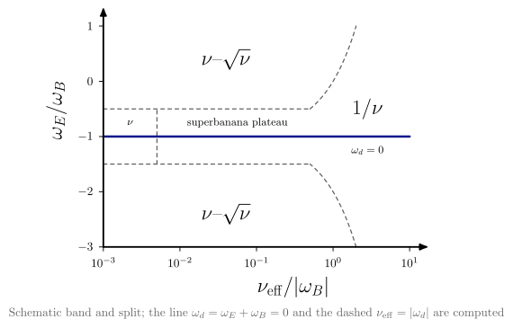
vaft.diagram.ntv_precession_regimes()Collisionality alone does not fix the NTV regime: the precession plane.
vaft.diagram.ntv_precession_regimes(*, omega_magnetic=1.0, band=0.5, labels=True)Show source vaft/diagram/_transport_regimes.py, lines 139–199
def ntv_precession_regimes(*, omega_magnetic: float = 1.0, band: float = 0.5, labels: bool = True) -> Diagram:
r"""Collisionality alone does not fix the NTV regime: the precession plane.
Axes $\nu_\mathrm{eff}/|\omega_B|$ (log) and $\omega_E/\omega_B$ for a
magnetic precession $\omega_B$ = ``omega_magnetic``, both along the
plasma current. From ``ntv_precession_frequency``: the resonance line
$\omega_d = 0$ and the ordering $\nu_\mathrm{eff} = |\omega_d|$ (dashed)
between $1/\nu$ (collisions faster than precession, right) and
$\nu$--$\sqrt\nu$ (left). Schematic: the resonant band
$|\omega_d| \lesssim$ ``band`` $\cdot|\omega_B|$ -- the spread of
$\omega_B$ over trapped pitch, whose zero some particles then cross --
holds the superbanana plateau for $\nu_\mathrm{eff} \lesssim |\omega_B|$
and the superbanana $\nu$ regime at the lowest collisionality; both
band edges and the split are illustrative.
"""
labels = _check_labels(labels)
if not (np.isfinite(omega_magnetic) and omega_magnetic != 0.0):
raise ValueError(f"omega_magnetic must be finite and non-zero, not {omega_magnetic!r}")
if not 0.0 < band < 1.0:
raise ValueError(f"band must lie in (0, 1), not {band!r}")
wb = float(omega_magnetic)
# the resonance: omega_d = omega_E + omega_B is linear in omega_E; locate its zero from the formula
slope = ntv_precession_frequency(1.0, 0.0)
y_res = -ntv_precession_frequency(0.0, wb) / (slope * wb)
x_band = float(np.log10(band))
y = np.linspace(y_res - 2.0, y_res + 2.0, 401)
omega_d = ntv_precession_frequency(y * wb, wb)
with np.errstate(divide="ignore"):
x_order = np.log10(np.abs(omega_d / wb))
# the ordering is drawn outside the resonant band only
upper, lower = (y - y_res) >= band, (y_res - y) >= band
chart = Chart(x_range=(-3.0, 1.0), y_range=(y_res - 2.0, y_res + 2.0))
x_sb = -2.3
chart.curves.update({
"resonance": np.array([[-3.0, y_res], [1.0, y_res]]),
"ordering_upper": np.stack([x_order[upper], y[upper]], axis=-1),
"ordering_lower": np.stack([x_order[lower], y[lower]], axis=-1),
"band_upper": np.array([[-3.0, y_res + band], [x_band, y_res + band]]),
"band_lower": np.array([[-3.0, y_res - band], [x_band, y_res - band]]),
"band_split": np.array([[x_sb, y_res - band], [x_sb, y_res + band]]),
})
chart.labels.update({"one_over_nu": (0.45, y_res + 0.5), "nonres_upper": (-1.4, y_res + 1.4),
"nonres_lower": (-1.4, y_res - 1.4), "sbp": (-1.25, y_res + 0.25),
"superbanana_nu": (-2.65, y_res + 0.25), "resonance": (0.45, y_res - 0.25)})
chart.parameters.update({"omega_magnetic": wb, "omega_exb_at_resonance": y_res * wb, "band": band})
x_ticks, x_text = _decades(-3, 1)
y_ticks = [float(v) for v in np.arange(np.ceil(y_res - 2.0), np.floor(y_res + 2.0) + 1.0)]
scene = render_chart(
chart,
x_label="$\\nu_\\mathrm{eff}/|\\omega_B|$",
y_label="$\\omega_E/\\omega_B$",
curve_styles={"ordering_upper": "approx", "ordering_lower": "approx", "band_upper": "approx",
"band_lower": "approx", "band_split": "approx", "resonance": "boundary"},
region_text={"one_over_nu": "$1/\\nu$", "nonres_upper": "$\\nu$--$\\sqrt\\nu$",
"nonres_lower": "$\\nu$--$\\sqrt\\nu$", "sbp": "\\small superbanana plateau",
"superbanana_nu": "\\small $\\nu$", "resonance": "\\small $\\omega_d = 0$"} if labels else {},
x_ticks=x_ticks, x_tick_text=x_text, y_ticks=y_ticks,
note=("Schematic band and split; the line $\\omega_d = \\omega_E + \\omega_B = 0$ and the dashed "
"$\\nu_\\mathrm{eff} = |\\omega_d|$ are computed" if labels else ""),
)
return Diagram("ntv_precession_regimes", scene, model=chart)Formats .svg .tex .pdf the SVG above is committed; build the others locally
import vaft.diagram
d = vaft.diagram.ntv_precession_regimes()
d.tikz # the TikZ document as text
d.save("ntv_precession_regimes.svg") # rendered vector image, the canonical artifact; needs latex, dvisvgm
d.save("ntv_precession_regimes.tex") # the complete TikZ document, the text source
d.save("ntv_precession_regimes.pdf") # vector PDF; needs pdflatexFormula functions referenced:
ntv.ntv_precession_frequency
Wall conditioning: baking, glow-discharge cleaning and boronization as wall-state transitions
Module vaft.diagram._wall_conditioning
wall_conditioning_baking
1 asset
source
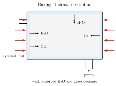
vaft.diagram.wall_conditioning_baking()Baking: external heat desorbs water and gases from the wall into the pump.
vaft.diagram.wall_conditioning_baking(*, temperature=None, temperature_unit='K', temperature_source=None, labels=True)Show source vaft/diagram/_wall_conditioning.py, lines 202–219
def wall_conditioning_baking(*, temperature: Optional[float] = None, temperature_unit: str = "K",
temperature_source: Optional[str] = None, labels: bool = True) -> Diagram:
r"""Baking: external heat desorbs water and gases from the wall into the pump.
Thermal desorption only -- no glow, anode, ion bombardment or coating.
The desorbed species are examples. The wall temperature is drawn only if
given, in ``temperature_unit`` (``"K"`` or ``"degC"``), and then only with
its ``temperature_source``; no "typical" baking temperature is built in.
"""
labels = _check_labels(labels)
if temperature_unit not in TEMPERATURE_UNITS:
raise ValueError(f"temperature_unit must be one of {tuple(TEMPERATURE_UNITS)}, not {temperature_unit!r}")
temperature = _quantity(temperature, temperature_source, "temperature")
items = _baking_items(0.0, labels, temperature, temperature_unit, temperature_source)
return Diagram("wall_conditioning_baking", Scene(tuple(items)),
model={"stage": "baking", "state_change": WALL_STATE_CHANGE["baking"], "temperature": temperature,
"temperature_unit": temperature_unit if temperature is not None else None,
"temperature_source": temperature_source})Formats .svg .tex .pdf the SVG above is committed; build the others locally
import vaft.diagram
d = vaft.diagram.wall_conditioning_baking()
d.tikz # the TikZ document as text
d.save("wall_conditioning_baking.svg") # rendered vector image, the canonical artifact; needs latex, dvisvgm
d.save("wall_conditioning_baking.tex") # the complete TikZ document, the text source
d.save("wall_conditioning_baking.pdf") # vector PDF; needs pdflatexwall_conditioning_gdc
2 assets
source
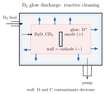
vaft.diagram.wall_conditioning_gdc(gas='D2')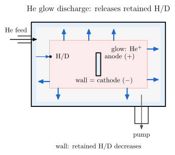
vaft.diagram.wall_conditioning_gdc(gas='He')Glow-discharge cleaning: one apparatus template, gas-specific content.
vaft.diagram.wall_conditioning_gdc(gas='D2', *, labels=True)Show source vaft/diagram/_wall_conditioning.py, lines 222–238
def wall_conditioning_gdc(gas: str = "D2", *, labels: bool = True) -> Diagram:
r"""Glow-discharge cleaning: one apparatus template, gas-specific content.
Gas feed, glow, anode, the wall as cathode, ions accelerated across the
cathode sheath onto the wall, and the pump are shared. H$_2$ or D$_2$:
reactive cleaning -- O and C contaminants leave as volatile products
(examples isotope-consistent with the feed: H$_2$O/CH$_4$ or D$_2$O/CD$_4$).
He: He$^+$ bombardment releases hydrogen isotopes retained in the wall
(ion-induced desorption), drawn with its own arrow style -- no chemistry,
a different purpose.
"""
if gas not in GASES:
raise ValueError(f"gas must be one of {GASES}, not {gas!r}")
labels = _check_labels(labels)
stage = f"{gas}_gdc"
return Diagram("wall_conditioning_gdc", Scene(tuple(_gdc_items(0.0, gas, labels))),
model={"stage": stage, "gas": gas, "state_change": WALL_STATE_CHANGE[stage]})Formats .svg .tex .pdf the SVG above is committed; build the others locally
import vaft.diagram
d = vaft.diagram.wall_conditioning_gdc(gas='D2')
d.tikz # the TikZ document as text
d.save("wall_conditioning_gdc_deuterium.svg") # rendered vector image, the canonical artifact; needs latex, dvisvgm
d.save("wall_conditioning_gdc_deuterium.tex") # the complete TikZ document, the text source
d.save("wall_conditioning_gdc_deuterium.pdf") # vector PDF; needs pdflatexwall_conditioning_boronization
1 asset
source
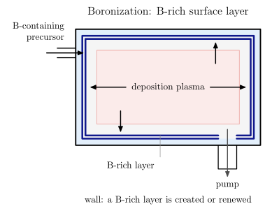
vaft.diagram.wall_conditioning_boronization()Boronization: a B-containing precursor in a deposition plasma coats the wall.
vaft.diagram.wall_conditioning_boronization(*, precursor=None, thickness_nm=None, thickness_source=None, labels=True)Show source vaft/diagram/_wall_conditioning.py, lines 241–258
def wall_conditioning_boronization(*, precursor: Optional[str] = None, thickness_nm: Optional[float] = None,
thickness_source: Optional[str] = None, labels: bool = True) -> Diagram:
r"""Boronization: a B-containing precursor in a deposition plasma coats the wall.
The generic diagram names no precursor ("B-containing precursor");
``precursor="B$_2$H$_6$"`` (or another) is annotated when given. The layer
thickness is drawn only with its source. A surface-state change rather
than cleaning: the B-rich layer getters oxygen and covers high-Z
surfaces, and it is what the plasma then sees.
"""
labels = _check_labels(labels)
if precursor is not None and (not isinstance(precursor, str) or not precursor):
raise ValueError(f"precursor must be a non-empty string, not {precursor!r}")
thickness_nm = _quantity(thickness_nm, thickness_source, "thickness_nm")
items = _boronization_items(0.0, labels, precursor, thickness_nm, thickness_source)
return Diagram("wall_conditioning_boronization", Scene(tuple(items)),
model={"stage": "boronization", "state_change": WALL_STATE_CHANGE["boronization"],
"precursor": precursor, "thickness_nm": thickness_nm, "thickness_source": thickness_source})Formats .svg .tex .pdf the SVG above is committed; build the others locally
import vaft.diagram
d = vaft.diagram.wall_conditioning_boronization()
d.tikz # the TikZ document as text
d.save("wall_conditioning_boronization.svg") # rendered vector image, the canonical artifact; needs latex, dvisvgm
d.save("wall_conditioning_boronization.tex") # the complete TikZ document, the text source
d.save("wall_conditioning_boronization.pdf") # vector PDF; needs pdflatexwall_conditioning_sequence
1 asset
source

vaft.diagram.wall_conditioning_sequence()Conditioning stages in order, each a transition of the wall state.
vaft.diagram.wall_conditioning_sequence(stages=('baking', 'D2_gdc', 'He_gdc', 'boronization'), *, plasma_operation=True, labels=True)Show source vaft/diagram/_wall_conditioning.py, lines 273–306
def wall_conditioning_sequence(stages: Sequence[str] = ("baking", "D2_gdc", "He_gdc", "boronization"), *,
plasma_operation: bool = True, labels: bool = True) -> Diagram:
r"""Conditioning stages in order, each a transition of the wall state.
``stages`` from ``STAGES``: ``"baking"``, ``"H2_gdc"``, ``"D2_gdc"``,
``"He_gdc"``, ``"boronization"``. Each panel is the corresponding
single-stage diagram without quantities; arrows between them are
wall-state transitions $S^{(k)} \to S^{(k+1)}$. With ``plasma_operation``
a last arrow hands the conditioned wall to plasma operation, where its
response is plasma-wall interaction. The order is the caller's, not a
recommended procedure.
"""
labels = _check_labels(labels)
stages = tuple(stages)
if not stages or any(s not in STAGES for s in stages):
raise ValueError(f"stages must be a non-empty sequence of {STAGES}, not {stages!r}")
items: List = []
for k, stage in enumerate(stages):
x0 = k * SEQUENCE_PITCH
items += _stage_items(stage, x0, labels)
if k:
items.append(Arrow((x0 - 3.7, _H / 2), (x0 - 1.6, _H / 2), "connector", role="transition"))
if labels:
items.append(Label((x0 - 2.65, _H / 2 + 0.15), f"$S^{{({k - 1})}} \\to S^{{({k})}}$",
"small label", anchor="south", role="transition"))
if plasma_operation:
x_end = (len(stages) - 1) * SEQUENCE_PITCH + _W
items.append(Arrow((x_end + 1.3, _H / 2), (x_end + 3.0, _H / 2), "connector", role="plasma_operation"))
if labels:
items.append(Label((x_end + 3.1, _H / 2), "\\begin{tabular}{l}plasma\\\\operation\\end{tabular}",
"small label", anchor="west", role="plasma_operation"))
return Diagram("wall_conditioning_sequence", Scene(tuple(items)),
model={"stages": stages, "state_changes": tuple(WALL_STATE_CHANGE[s] for s in stages),
"plasma_operation": plasma_operation})Formats .svg .tex .pdf the SVG above is committed; build the others locally
import vaft.diagram
d = vaft.diagram.wall_conditioning_sequence()
d.tikz # the TikZ document as text
d.save("wall_conditioning_sequence.svg") # rendered vector image, the canonical artifact; needs latex, dvisvgm
d.save("wall_conditioning_sequence.tex") # the complete TikZ document, the text source
d.save("wall_conditioning_sequence.pdf") # vector PDF; needs pdflatexField-aligned coordinates, flux tubes, shear and the ballooning eigenfunction (#1075, part 2)
Module vaft.diagram._field_aligned
field_aligned_basis
1 asset
source
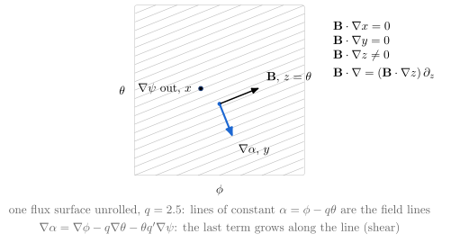
vaft.diagram.field_aligned_basis()Why a field-aligned system is simple: two coordinates are constant along the field, one follows it.
vaft.diagram.field_aligned_basis(q=2.5, *, labels=True)Show source vaft/diagram/_field_aligned.py, lines 67–132
def field_aligned_basis(q: float = 2.5, *, labels: bool = True) -> Diagram:
r"""Why a field-aligned system is simple: two coordinates are constant along the field, one follows it.
The flux surface unrolled onto $(\phi, \theta) \in [0, 2\pi)^2$; its field
lines are the lines of constant $\alpha = \phi - q\theta$ (``field_line_label``),
here eight of them. At one point: $\mathbf B$ along the line, the
components $\partial_i\alpha = (1, -q)$ across it, $\nabla\psi$ out of
the page. The right angle is drawn in $(\phi, \theta)$ coordinate space:
$\mathbf B\cdot\nabla\alpha = B^\phi\partial_\phi\alpha + B^\theta\partial_\theta\alpha
= 0$ pairs contravariant with covariant components and holds with any
metric, while the true gradient $g^{ij}\partial_j\alpha$ is not at right
angles on the page. It is the in-surface part at $\theta = 0$ only:
$\nabla\alpha = \nabla\phi - q\nabla\theta - \theta q'\nabla\psi$ has a
radial part that grows secularly along the line -- the magnetic shear of
``magnetic_shear_field_aligned``.
With $x = \psi$, $y = \alpha$, $z = \theta$: $\mathbf B\cdot\nabla x = 0$,
$\mathbf B\cdot\nabla y = 0$, $\mathbf B\cdot\nabla z \ne 0$, so the parallel
derivative is one partial derivative.
"""
labels = _check_labels(labels)
if not q > 0:
raise ValueError(f"q must be positive, not {q!r}")
size = 5.0
sc = size / (2.0 * math.pi)
items: List = [Polyline.of([(0, 0), (size, 0), (size, size), (0, size)], "inset frame", role="surface",
closed=True)]
theta = np.linspace(0.0, 2.0 * math.pi, 400)
for k in range(8):
alpha0 = 2.0 * math.pi * k / 8
# alpha = phi - q theta = alpha0 -> phi = alpha0 + q theta, wrapped into the square
phi = alpha0 + q * theta
wrapped = np.mod(phi, 2.0 * math.pi)
breaks = np.where(np.diff(wrapped) < 0)[0] + 1
for seg_phi, seg_theta in zip(np.split(wrapped, breaks), np.split(theta, breaks)):
if len(seg_phi) > 1:
items.append(Polyline.of(np.stack([seg_phi * sc, seg_theta * sc], -1), "surface",
role="field_line"))
# at a point: B^i along (q, 1) in (phi, theta); the covariant d_i alpha = (1, -q): B^i d_i alpha = 0
P = np.array([0.5 * size, 0.42 * size])
b = np.array([q, 1.0]) / math.hypot(q, 1.0)
g = np.array([1.0, -q]) / math.hypot(1.0, q)
items += [Marker(tuple(P), "o", "opoint", role="point"),
Arrow(tuple(P), tuple(P + 1.3 * b), "vector", role="B"),
Arrow(tuple(P), tuple(P + 1.1 * g), "drift ion", role="grad_alpha"),
Marker(tuple(P + np.array([-0.55, 0.45])), "o", "xpoint", role="grad_psi")]
if labels:
items += [Label(tuple(P + 1.35 * b), "$\\mathbf B$, $z = \\theta$", "small label", anchor="south west",
role="B"),
Label(tuple(P + 1.15 * g), "$\\nabla\\alpha$, $y$", "small label", anchor="north west",
role="grad_alpha"),
Label(tuple(P + np.array([-0.7, 0.45])), "$\\nabla\\psi$ out, $x$", "small label", anchor="east",
role="grad_psi"),
Label((size / 2, -0.15), "$\\phi$", "small label", anchor="north", role="axes"),
Label((-0.15, size / 2), "$\\theta$", "small label", anchor="east", role="axes"),
Label((size + 0.5, size - 0.3),
"\\begin{tabular}{l}$\\mathbf B\\cdot\\nabla x = 0$\\\\$\\mathbf B\\cdot\\nabla y = 0$\\\\"
"$\\mathbf B\\cdot\\nabla z \\neq 0$\\\\[3pt]$\\mathbf B\\cdot\\nabla = "
"(\\mathbf B\\cdot\\nabla z)\\,\\partial_z$\\end{tabular}", "small label", anchor="north west",
role="conditions"),
Label((size / 2, -0.75), f"one flux surface unrolled, $q = {q:g}$: lines of constant "
"$\\alpha = \\phi - q\\theta$ are the field lines", "note", anchor="north", role="note")]
if labels:
items.append(Label((size / 2, -1.25), "$\\nabla\\alpha = \\nabla\\phi - q\\nabla\\theta - \\theta q'\\nabla\\psi$: "
"the last term grows along the line (shear)", "note", anchor="north", role="secular"))
return Diagram("field_aligned_basis", Scene(tuple(items)),
model={"q": q, "B_direction": tuple(b), "grad_alpha_direction": tuple(g)})Formats .svg .tex .pdf the SVG above is committed; build the others locally
import vaft.diagram
d = vaft.diagram.field_aligned_basis()
d.tikz # the TikZ document as text
d.save("field_aligned_basis.svg") # rendered vector image, the canonical artifact; needs latex, dvisvgm
d.save("field_aligned_basis.tex") # the complete TikZ document, the text source
d.save("field_aligned_basis.pdf") # vector PDF; needs pdflatexflux_tube_patch
1 asset
source
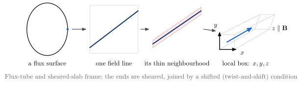
vaft.diagram.flux_tube_patch()From a tokamak flux surface to a local flux tube: one surface, one line, its neighbourhood, a box.
vaft.diagram.flux_tube_patch(*, labels=True)Show source vaft/diagram/_field_aligned.py, lines 135–197
def flux_tube_patch(*, labels: bool = True) -> Diagram:
r"""From a tokamak flux surface to a local flux tube: one surface, one line, its neighbourhood, a box.
A concept sequence: a flux surface in the poloidal cross-section; one of
its field lines; the thin radial and binormal neighbourhood that follows
it; and the local box with $x$ radial, $y$ binormal, $z$ along
$\mathbf B$ -- the frame of local gyrokinetic flux-tube codes and of the
sheared slab. The box's ends are sheared by the magnetic shear, so they
are joined by a shifted, not a plain periodic, condition (twist and
shift; not derived here).
"""
labels = _check_labels(labels)
items: List = []
# 1. cross-section: one flux surface and a point on it
t = np.linspace(0.0, 2.0 * math.pi, 121)
c1 = np.array([1.3, 1.3])
items.append(Polyline.of(c1 + 1.1 * np.stack([np.cos(t), 1.3 * np.sin(t)], -1), "lcfs", role="flux_surface",
closed=True))
items.append(Marker(tuple(c1 + np.array([1.1, 0.0])), "o", "opoint", role="point"))
# 2. the surface unrolled with one field line
x2 = 3.6
items.append(Polyline.of([(x2, 0.0), (x2 + 2.6, 0.0), (x2 + 2.6, 2.6), (x2, 2.6)], "inset frame",
role="unrolled_surface", closed=True))
line = np.array([[x2, 0.3], [x2 + 2.6, 2.3]])
items.append(Polyline.of(line, "field line", role="field_line"))
# 3. the thin neighbourhood around the line
x3 = 7.0
items.append(Polyline.of([(x3, 0.3), (x3 + 2.6, 2.1), (x3 + 2.6, 2.5), (x3, 0.7)], "layer", role="neighbourhood",
closed=True))
items.append(Polyline.of([(x3, 0.5), (x3 + 2.6, 2.3)], "field line", role="field_line"))
# 4. the local box in oblique projection: an x-y end face, elongated along z; the far face is
# sheared (its x position shifts with y) relative to the near one
x4 = 10.6
o = np.array([x4, 0.2])
ex, ey, ez = np.array([0.8, 0.0]), np.array([0.0, 0.8]), np.array([1.9, 1.1])
shear_shift = 0.35 * ex
near = [o, o + ex, o + ex + ey, o + ey]
far = [o + ez, o + ez + ex, o + ez + ex + ey + shear_shift, o + ez + ey + shear_shift]
items.append(Polyline.of(near, "surface", role="flux_tube_end", closed=True))
items.append(Polyline.of(far, "surface", role="flux_tube_end", closed=True))
for a, b in zip(near, far):
items.append(Polyline.of([a, b], "surface", role="flux_tube"))
items += [Arrow(tuple(o), tuple(o + 1.2 * ex), "vector", role="x_axis"),
Arrow(tuple(o), tuple(o + 1.25 * ey), "vector", role="y_axis"),
Arrow(tuple(o + 0.5 * (ex + ey)), tuple(o + 0.5 * (ex + ey) + 0.75 * ez), "drift ion",
role="z_axis")]
for a, b in ((c1 + np.array([1.35, 0.0]), (x2 - 0.15, 1.3)), ((x2 + 2.75, 1.3), (x3 - 0.15, 1.3)),
((x3 + 2.75, 1.3), (x4 - 0.15, 1.2))):
items.append(Arrow(tuple(a), tuple(b), "connector", role="step"))
if labels:
items += [Label((c1[0], -0.3), "a flux surface", "small label", anchor="north", role="flux_surface"),
Label((x2 + 1.3, -0.3), "one field line", "small label", anchor="north", role="field_line"),
Label((x3 + 1.3, -0.3), "its thin neighbourhood", "small label", anchor="north",
role="neighbourhood"),
Label((x4 + 1.4, -0.3), "local box: $x, y, z$", "small label", anchor="north", role="flux_tube"),
Label(tuple(o + 1.25 * ex), "$x$", "small label", anchor="north west", role="x_axis"),
Label(tuple(o + 1.3 * ey), "$y$", "small label", anchor="south east", role="y_axis"),
Label(tuple(o + ez + ex + 0.05 * ey), "$z \\parallel \\mathbf B$", "small label",
anchor="west", role="z_axis"),
Label((6.9, -1.0), "Flux-tube and sheared-slab frame; the ends are sheared, joined by a shifted "
"(twist-and-shift) condition", "note", anchor="north", role="note")]
return Diagram("flux_tube_patch", Scene(tuple(items)), model={"steps": ("surface", "field_line",
"neighbourhood", "flux_tube")})Formats .svg .tex .pdf the SVG above is committed; build the others locally
import vaft.diagram
d = vaft.diagram.flux_tube_patch()
d.tikz # the TikZ document as text
d.save("flux_tube_patch.svg") # rendered vector image, the canonical artifact; needs latex, dvisvgm
d.save("flux_tube_patch.tex") # the complete TikZ document, the text source
d.save("flux_tube_patch.pdf") # vector PDF; needs pdflatexmagnetic_shear_field_aligned
1 asset
source
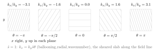
vaft.diagram.magnetic_shear_field_aligned()Magnetic shear rotates the phase fronts of a field-aligned mode as it is followed along the line.
vaft.diagram.magnetic_shear_field_aligned(*, shear=1.0, labels=True)Show source vaft/diagram/_field_aligned.py, lines 200–250
def magnetic_shear_field_aligned(*, shear: float = 1.0, labels: bool = True) -> Diagram:
r"""Magnetic shear rotates the phase fronts of a field-aligned mode as it is followed along the line.
Five local $(x, y)$ planes at $z = \theta = -\pi, -\pi/2, 0, \pi/2, \pi$
with the fronts of a mode of fixed $k_y$: the radial wavenumber is
``ballooning_radial_wavenumber`` ($\alpha = 0$, $\theta_0 = 0$),
$k_x = k_y\hat s\theta$, so the fronts tilt by $\arctan(\hat s\theta)$ -- the
sheared-slab $k_x(z) = k_{x0} + k_y\hat s z$ seen in the tokamak. The
binormal period $2\pi/k_y$ is the same in every plane (the fronts cross
each vertical line at the same spacing), so the spacing across the fronts
shrinks as $1/\sqrt{1 + \hat s^2\theta^2}$: $k_\perp$ grows along the line,
the $(1 + \Lambda^2)$ of line bending and inertia.
"""
labels = _check_labels(labels)
k_y, size, pitch, wavelength_y = 1.0, 2.0, 2.8, 0.6
zs = [-math.pi, -0.5 * math.pi, 0.0, 0.5 * math.pi, math.pi]
items: List = []
kxs = []
for i, z in enumerate(zs):
k_x = float(ballooning_radial_wavenumber(k_y, shear, z))
kxs.append(k_x)
x0 = i * pitch
items.append(Polyline.of([(x0, 0), (x0 + size, 0), (x0 + size, size), (x0, size)], "inset frame",
role="plane", closed=True))
# fronts k_x x + k_y y = const, one per binormal wavelength along y, clipped to the square
kk = math.hypot(k_x, k_y)
d = np.array([k_y, -k_x]) / kk # along a front, normal to (k_x, k_y)
c = np.array([x0 + size / 2, size / 2])
reach = 0.5 * size * (1.0 + abs(k_x / k_y)) # y-span of the fronts that cross the square
n_front = int(math.ceil(reach / wavelength_y))
for j in range(-n_front, n_front + 1):
p0 = c + np.array([0.0, j * wavelength_y])
seg = np.array([p0 - 2 * size * d, p0 + 2 * size * d])
clipped = _clip_segment(seg, (x0, 0.0, x0 + size, size))
if clipped is not None:
items.append(Polyline.of(clipped, "surface", role=f"front_{i}"))
if labels:
items.append(Label((x0 + size / 2, -0.15), f"$\\theta = {_pi_text(z)}$", "small label", anchor="north",
role="plane"))
items.append(Label((x0 + size / 2, size + 0.1), f"$k_x/k_y = {k_x / k_y:.1f}$", "small label",
anchor="south", role="kx"))
if labels:
items += [Label((-0.15, size / 2), "$y$", "small label", anchor="east", role="axes"),
Label((0.2, -0.65), "$x$ right, $y$ up in each plane", "small label", anchor="north west",
role="axes"),
Label((2 * pitch + size / 2, -1.2), f"$\\hat s = {shear:g}$: $k_x = k_y\\hat s\\theta$ "
"(ballooning\\_radial\\_wavenumber), the sheared slab along the field line", "note",
anchor="north", role="note")]
return Diagram("magnetic_shear_field_aligned", Scene(tuple(items)),
model={"shear": shear, "theta": tuple(zs), "k_x": tuple(kxs), "k_y": k_y,
"wavelength_y": wavelength_y})Formats .svg .tex .pdf the SVG above is committed; build the others locally
import vaft.diagram
d = vaft.diagram.magnetic_shear_field_aligned()
d.tikz # the TikZ document as text
d.save("magnetic_shear_field_aligned.svg") # rendered vector image, the canonical artifact; needs latex, dvisvgm
d.save("magnetic_shear_field_aligned.tex") # the complete TikZ document, the text source
d.save("magnetic_shear_field_aligned.pdf") # vector PDF; needs pdflatexFormula functions referenced:
stability.ballooning_radial_wavenumber
ballooning_eigenfunction
1 asset
source
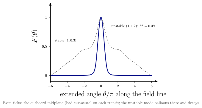
vaft.diagram.ballooning_eigenfunction()A ballooning mode: localised on the extended angle where the curvature is bad.
vaft.diagram.ballooning_eigenfunction(*, labels=True)Show source vaft/diagram/_field_aligned.py, lines 279–312
def ballooning_eigenfunction(*, labels: bool = True) -> Diagram:
r"""A ballooning mode: localised on the extended angle where the curvature is bad.
``s_alpha_ballooning_eigenmode`` on $[-6\pi, 6\pi]$ with vanishing ends:
at $(s, \alpha) = (1, 1.2)$, beyond the first stability boundary, the
most unstable mode ($\hat\gamma^2 > 0$) peaks at $\theta = 0$ -- the
outboard midplane, bad curvature -- and decays within a few poloidal
transits; at $(1, 0.3)$, stable, the top eigenvector is the discretised
continuum and fills the interval. Ticks at $\theta = 0, \pm 2\pi, \ldots$
are the outboard midplane on successive transits, $\pm\pi, \pm 3\pi, \ldots$
the inboard one. The extended-angle localisation is the ballooning
boundary condition; flux-tube codes instead join the sheared ends.
"""
labels = _check_labels(labels)
g_u, th, F_u = s_alpha_ballooning_eigenmode(*UNSTABLE)
g_s, _, F_s = s_alpha_ballooning_eigenmode(*STABLE)
x = th / math.pi
chart = Chart(x_range=(float(x[0]), float(x[-1])), y_range=(-0.1, 1.15))
chart.curves["unstable"] = np.stack([x, F_u], -1)
chart.curves["stable"] = np.stack([x, F_s], -1)
chart.labels.update({"unstable": (3.8, 0.85), "stable": (-4.2, 0.6)})
chart.parameters.update({"growth_rate_squared_unstable": g_u, "growth_rate_squared_stable": g_s,
"unstable": UNSTABLE, "stable": STABLE})
ticks = [float(k) for k in range(-6, 7, 2)]
scene = render_chart(
chart, x_label="extended angle $\\theta/\\pi$ along the field line", y_label="$F(\\theta)$",
curve_styles={"stable": "approx", "unstable": "boundary"},
region_text={"unstable": f"\\small unstable $(1, 1.2)$: $\\hat\\gamma^2 = {g_u:.2f}$",
"stable": "\\small stable $(1, 0.3)$"} if labels else {},
x_ticks=ticks, x_tick_text=[f"${int(t)}$" for t in ticks], y_ticks=[0.0, 0.5, 1.0],
note=("Even ticks: the outboard midplane (bad curvature) on each transit; the unstable mode balloons "
"there and decays" if labels else ""),
)
return Diagram("ballooning_eigenfunction", scene, model=chart)Formats .svg .tex .pdf the SVG above is committed; build the others locally
import vaft.diagram
d = vaft.diagram.ballooning_eigenfunction()
d.tikz # the TikZ document as text
d.save("ballooning_eigenfunction.svg") # rendered vector image, the canonical artifact; needs latex, dvisvgm
d.save("ballooning_eigenfunction.tex") # the complete TikZ document, the text source
d.save("ballooning_eigenfunction.pdf") # vector PDF; needs pdflatexFormula functions referenced:
stability.s_alpha_ballooning_eigenmode
ballooning_transit_map
1 asset
source
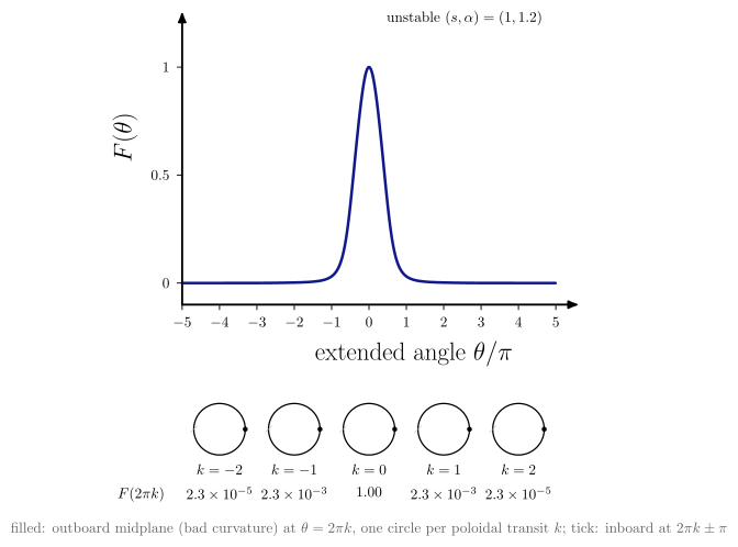
vaft.diagram.ballooning_transit_map()Where the extended angle is in the cross-section: one poloidal circle per transit.
vaft.diagram.ballooning_transit_map(*, transits=2, labels=True)Show source vaft/diagram/_field_aligned.py, lines 327–380
def ballooning_transit_map(*, transits: int = 2, labels: bool = True) -> Diagram:
r"""Where the extended angle is in the cross-section: one poloidal circle per transit.
Top, the unstable eigenfunction of ``ballooning_eigenfunction``
($(s, \alpha) = (1, 1.2)$) on $|\theta| \le (2\,\mathrm{transits} + 1)\pi$.
Below, one poloidal cross-section per transit $k$, centred under
$\theta = 2\pi k$: the field line crosses the outboard midplane (bad
curvature, filled) at $\theta = 2\pi k$ and the inboard one (good
curvature, open) at $2\pi k \pm \pi$. The number by each outboard point is
$F(2\pi k)$: the same geometric point, visited again on every transit,
carries less of the mode each time -- why the mode "balloons" on the
outboard side of one transit.
"""
labels = _check_labels(labels)
transits = _count(transits, "transits", 1, 3)
# the box must reach past the drawn range: its Dirichlet ends are a numerical condition, not the mode
_, th, F = s_alpha_ballooning_eigenmode(*UNSTABLE, theta_max=max(6.0, 2.0 * transits + 2.0) * math.pi)
F = F / np.max(np.abs(F))
half = (2 * transits + 1)
keep = np.abs(th) <= half * math.pi
x = th[keep] / math.pi
chart = Chart(x_range=(-float(half), float(half)), y_range=(-0.1, 1.15))
chart.curves["unstable"] = np.stack([x, F[keep]], -1)
ticks = [float(k) for k in range(-half, half + 1)]
scene = render_chart(
chart, x_label="extended angle $\\theta/\\pi$", y_label="$F(\\theta)$",
curve_styles={"unstable": "boundary"}, region_text={},
x_ticks=ticks, x_tick_text=[f"${int(t)}$" for t in ticks], y_ticks=[0.0, 0.5, 1.0])
items: List = list(scene.items)
ks = list(range(-transits, transits + 1))
amplitude = {k: float(np.interp(2.0 * k * math.pi, th, F)) for k in ks}
rad, y0 = 0.62, -3.0
for k in ks:
cx = float(chart.to_cm(np.array([2.0 * k, 0.0]))[0])
t = np.linspace(0.0, 2.0 * math.pi, 73)
items.append(Polyline.of(np.stack([cx + rad * np.cos(t), y0 + rad * np.sin(t)], -1), "lcfs",
role="cross_section", closed=True))
items.append(Marker((cx + rad, y0), "o", "star", role="outboard"))
items.append(Polyline.of([(cx - rad - 0.08, y0 - 0.08), (cx - rad + 0.08, y0 + 0.08)], "surface",
role="inboard"))
if labels:
items += [Label((cx, y0 - rad - 0.1), f"$k = {k}$", "small label", anchor="north", role="transit"),
Label((cx, y0 - rad - 0.65), _amplitude_text(amplitude[k]), "small label", anchor="north",
role="amplitude")]
if labels:
items += [Label((chart.to_cm(np.array([0.0, 1.0]))[0] + 0.3, 6.9),
"unstable $(s, \\alpha) = (1, 1.2)$", "small label", anchor="west", role="title"),
Label((-0.3, y0 - rad - 0.65), "$F(2\\pi k)$", "small label", anchor="north east",
role="amplitude"),
Label((4.5, y0 - 2.1), "filled: outboard midplane (bad curvature) at $\\theta = 2\\pi k$, "
"one circle per poloidal transit $k$; tick: inboard at $2\\pi k \\pm \\pi$", "note", anchor="north",
role="note")]
return Diagram("ballooning_transit_map", Scene(tuple(items)),
model={"transits": tuple(ks), "amplitude": amplitude, "unstable": UNSTABLE})Formats .svg .tex .pdf the SVG above is committed; build the others locally
import vaft.diagram
d = vaft.diagram.ballooning_transit_map()
d.tikz # the TikZ document as text
d.save("ballooning_transit_map.svg") # rendered vector image, the canonical artifact; needs latex, dvisvgm
d.save("ballooning_transit_map.tex") # the complete TikZ document, the text source
d.save("ballooning_transit_map.pdf") # vector PDF; needs pdflatexFormula functions referenced:
stability.s_alpha_ballooning_eigenmode
ballooning_boundary_conditions
1 asset
source
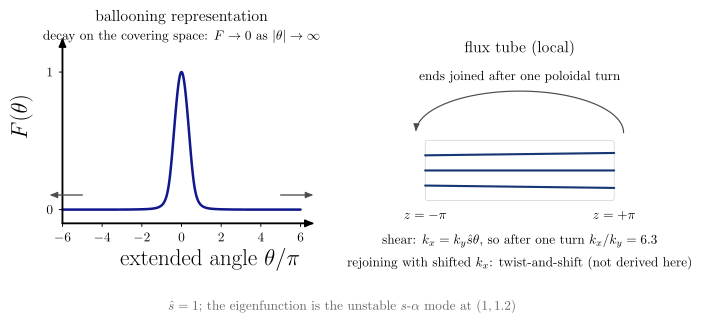
vaft.diagram.ballooning_boundary_conditions()Two ways to close the field line: decay on the covering space, or a sheared parallel join.
vaft.diagram.ballooning_boundary_conditions(*, shear=1.0, labels=True)Show source vaft/diagram/_field_aligned.py, lines 383–444
def ballooning_boundary_conditions(*, shear: float = 1.0, labels: bool = True) -> Diagram:
r"""Two ways to close the field line: decay on the covering space, or a sheared parallel join.
Left, the ballooning representation: the eigenfunction lives on the
extended angle $\theta \in (-\infty, \infty)$, the covering space of the
periodic poloidal angle, and the boundary condition is decay,
$F \to 0$ as $|\theta| \to \infty$ (the unstable mode of
``ballooning_eigenfunction``). Right, a flux-tube box of finite parallel
length: its two ends are the same poloidal position, joined after
following the line once round. Magnetic shear connects the two pictures:
a mode with $k_y$ has $k_x = k_y\hat s\theta$ (``ballooning_radial_wavenumber``),
so the end it rejoins has a shifted $k_x$ -- the twist-and-shift
condition, named here and not derived.
"""
labels = _check_labels(labels)
if isinstance(shear, bool) or not isinstance(shear, (int, float, np.floating, np.integer)) \
or not 0.1 <= float(shear) <= 3.0:
raise ValueError(f"shear must be a number from 0.1 to 3, not {shear!r}")
shear = float(shear)
_, th, F = s_alpha_ballooning_eigenmode(*UNSTABLE)
F = F / np.max(np.abs(F))
chart = Chart(x_range=(-6.0, 6.0), y_range=(-0.1, 1.15))
chart.curves["unstable"] = np.stack([th / math.pi, F], -1)
ticks = [-6.0, -4.0, -2.0, 0.0, 2.0, 4.0, 6.0]
scene = render_chart(chart, x_label="extended angle $\\theta/\\pi$", y_label="$F(\\theta)$",
curve_styles={"unstable": "boundary"}, region_text={}, x_ticks=ticks,
x_tick_text=[f"${int(t)}$" for t in ticks], y_ticks=[0.0, 1.0])
items: List = list(scene.transformed(scale=0.7).items)
for side in (-1, 1):
x = 0.7 * float(chart.to_cm(np.array([5.0 * side, 0.0]))[0])
items.append(Arrow((x, 0.75), (x + side * 0.9, 0.75), "connector", role="decay"))
# the flux tube: a box along z, both ends drawn, joined by a curved return with a shifted end
bx, by, length, width = 9.6, 0.6, 5.0, 1.6
items += [Polyline.of([(bx, by), (bx + length, by), (bx + length, by + width), (bx, by + width)], "inset frame",
role="flux_tube", closed=True)]
for f in (0.25, 0.5, 0.75):
y = by + f * width
items.append(Polyline.of([(bx, y), (bx + length, y + 0.25 * shear * (f - 0.5))], "field line",
role="field_line"))
t = np.linspace(0.0, math.pi, 50)
arc = np.stack([bx + length / 2 + (length / 2 + 0.25) * np.cos(t), by + width + 0.2 + 1.1 * np.sin(t)], -1)
items.append(Polyline.of(arc, "angle arc", role="parallel_join"))
k_x = float(ballooning_radial_wavenumber(1.0, shear, 2.0 * math.pi))
if labels:
items += [Label((0.7 * 4.5, 0.7 * 6.5 + 0.6), "ballooning representation", "label", anchor="south",
role="title"),
Label((bx + length / 2, 4.3), "flux tube (local)", "label", anchor="south", role="title"),
Label((0.7 * 4.5, 0.7 * 6.5 + 0.1), "decay on the covering space: $F \\to 0$ as "
"$|\\theta| \\to \\infty$", "small label", anchor="south", role="decay"),
Label((bx + length / 2, by + width + 1.4), "ends joined after one poloidal turn",
"small label", anchor="south", role="parallel_join"),
Label((bx, by - 0.15), "$z = -\\pi$", "small label", anchor="north", role="ends"),
Label((bx + length, by - 0.15), "$z = +\\pi$", "small label", anchor="north", role="ends"),
Label((bx + length / 2, by - 0.75),
f"shear: $k_x = k_y\\hat s\\theta$, so after one turn $k_x/k_y = {k_x:.1f}$",
"small label", anchor="north", role="shear"),
Label((bx + length / 2, by - 1.35), "rejoining with shifted $k_x$: twist-and-shift "
"(not derived here)", "small label", anchor="north", role="twist_and_shift"),
Label((7.4, -1.9), f"$\\hat s = {shear:g}$; the eigenfunction is the unstable "
"$s$-$\\alpha$ mode at $(1, 1.2)$", "note", anchor="north", role="note")]
return Diagram("ballooning_boundary_conditions", Scene(tuple(items)),
model={"shear": shear, "kx_after_one_turn": k_x, "unstable": UNSTABLE})Formats .svg .tex .pdf the SVG above is committed; build the others locally
import vaft.diagram
d = vaft.diagram.ballooning_boundary_conditions()
d.tikz # the TikZ document as text
d.save("ballooning_boundary_conditions.svg") # rendered vector image, the canonical artifact; needs latex, dvisvgm
d.save("ballooning_boundary_conditions.tex") # the complete TikZ document, the text source
d.save("ballooning_boundary_conditions.pdf") # vector PDF; needs pdflatexFormula functions referenced:
stability.ballooning_radial_wavenumber, stability.s_alpha_ballooning_eigenmode
field_aligned_xpoint_limitation
1 asset
source
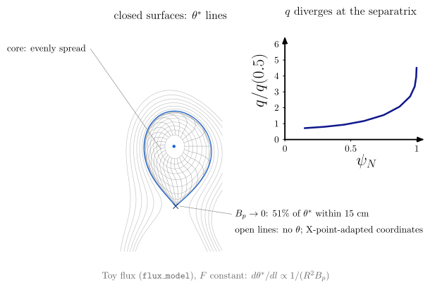
vaft.diagram.field_aligned_xpoint_limitation()Why field-aligned and flux coordinates fail at the X-point, on the diverted toy equilibrium.
vaft.diagram.field_aligned_xpoint_limitation(*, n_theta=24, labels=True)Show source vaft/diagram/_field_aligned.py, lines 488–552
def field_aligned_xpoint_limitation(*, n_theta: int = 24, labels: bool = True) -> Diagram:
r"""Why field-aligned and flux coordinates fail at the X-point, on the diverted toy equilibrium.
Left, lines of constant straight-field-line angle $\theta^*$ across the
closed surfaces of ``flux_model("diverted")`` ($n_\theta$ equal steps;
with $F$ constant $d\theta^*/dl \propto 1/(R^2B_p)$). In the core they
are evenly spread; towards the separatrix, where $B_p \to 0$ at the
X-point, $\theta^*$ is spent almost entirely near the X-point, so the
coordinate lines crowd into it and the cells elsewhere stretch -- a
strongly distorted metric. Outside the separatrix the field lines are
open (SOL, private flux): there is no poloidal angle at all, and
X-point-adapted or divertor coordinates are used instead. Right,
$q \propto \oint dl/(R^2B_p)$ relative to its value at $\psi_N = 0.5$,
diverging logarithmically as $\psi_N \to 1$ (cf. ``sfl_coordinate_validity``).
"""
labels = _check_labels(labels)
n_theta = _count(n_theta, "n_theta", 8, 64)
from ._gs_equilibrium import _cm, _surfaces, flux_model, lcfs
model = flux_model("diverted")
o = (0.0, 0.0)
points, loops = [], []
for psi_n in _XPOINT_SURFACES:
pts, loop = _straight_field_line_points(model, psi_n, n_theta)
points.append(pts)
loops.append(loop)
_, loop_half = _straight_field_line_points(model, 0.5, n_theta)
items: List = [Polyline.of(_cm(p, o), "surface", role="flux_surface", closed=True) for p in points]
items += [it for it in _surfaces(model, o) if it.role == "open_flux"]
stack = np.stack(points) # surface, theta, (R, Z)
for j in range(n_theta):
items.append(Polyline.of(_cm(stack[:, j, :], o), "mesh", role="theta_line"))
boundary = lcfs(model)
items += [Polyline.of(_cm(boundary, o), "separatrix", role="separatrix", closed=True),
Marker(tuple(_cm(model["x_point"], o)), "x", "xpoint", role="x_point"),
Marker(tuple(_cm(model["axis"], o)), "o", "opoint", role="axis")]
q_rel = np.array(loops) / loop_half
chart = Chart(x_range=(0.0, 1.0), y_range=(0.0, float(math.ceil(q_rel[-1] + 0.5))))
chart.curves["q"] = np.stack([np.array(_XPOINT_SURFACES), q_rel], -1)
q_scene = render_chart(chart, x_label="$\\psi_N$", y_label="$q / q(0.5)$", curve_styles={"q": "boundary"},
region_text={}, x_ticks=[0.0, 0.5, 1.0],
y_ticks=[float(v) for v in range(0, int(chart.y_range[1]) + 1)])
offset, scale = (7.6, 0.2), 0.55
items += list(q_scene.transformed(scale=scale, offset=offset).items)
# the fraction of the theta* range spent within 0.15 m of the X-point on the outermost surface
*_, near = _straight_field_line_points(model, _XPOINT_SURFACES[-1], n_theta, near=(model["x_point"], 0.15))
if labels:
xl = 5.6
items += [Label((3.3, 4.6), "closed surfaces: $\\theta^*$ lines", "label", anchor="south", role="title"),
Polyline.of([tuple(_cm(points[1][n_theta // 2], o)), (0.3, 3.6)], "leader line",
role="leader:core"),
Label((0.25, 3.6), "core: evenly spread", "small label", anchor="east", role="core"),
Polyline.of([tuple(_cm(model["x_point"], o) + [0.15, 0.0]), (xl, -2.6)], "leader line",
role="leader:x_point"),
Label((xl, -2.6), f"$B_p \\to 0$: {100 * near:.0f}\\% of $\\theta^*$ within 15 cm",
"small label", anchor="west", role="x_point"),
Label((xl, -3.2), "open lines: no $\\theta$; X-point-adapted coordinates", "small label",
anchor="west", role="open_flux"),
Label((offset[0] + scale * 4.5, offset[1] + scale * 6.5 + 0.9), "$q$ diverges at the separatrix",
"label", anchor="south", role="title"),
Label((5.0, -4.6), "Toy flux (\\texttt{flux\\_model}), $F$ constant: $d\\theta^*/dl \\propto "
"1/(R^2B_p)$", "note", anchor="north", role="note")]
return Diagram("field_aligned_xpoint_limitation", Scene(tuple(items)),
model={"psi_n": _XPOINT_SURFACES, "q_relative": tuple(float(v) for v in q_rel),
"fraction_near_x_point": near, "n_theta": n_theta})Formats .svg .tex .pdf the SVG above is committed; build the others locally
import vaft.diagram
d = vaft.diagram.field_aligned_xpoint_limitation()
d.tikz # the TikZ document as text
d.save("field_aligned_xpoint_limitation.svg") # rendered vector image, the canonical artifact; needs latex, dvisvgm
d.save("field_aligned_xpoint_limitation.tex") # the complete TikZ document, the text source
d.save("field_aligned_xpoint_limitation.pdf") # vector PDF; needs pdflatexSOL blobs and filaments: why a blob moves, how the current closes, how fast, and in which regime
Module vaft.diagram._blob
blob_polarization
2 assets
source
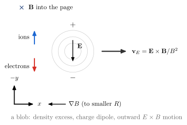
vaft.diagram.blob_polarization()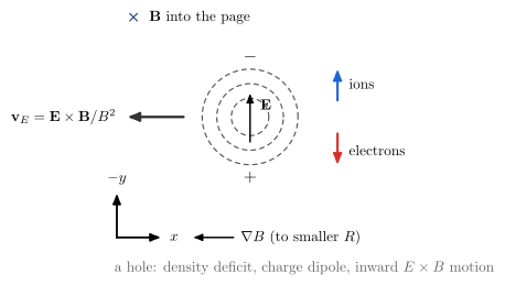
vaft.diagram.blob_polarization(perturbation='hole')Why a blob moves: curvature polarizes it into a dipole, and the dipole drifts it.
vaft.diagram.blob_polarization(*, perturbation='blob', labels=True)Show source vaft/diagram/_blob.py, lines 49–108
def blob_polarization(*, perturbation: str = "blob", labels: bool = True) -> Diagram:
r"""Why a blob moves: curvature polarizes it into a dipole, and the dipole drifts it.
In the $(x, y)$ plane with $\mathbf B$ into the page and $x$ outward
(larger $R$), $\nabla B$ points inward. The $\nabla B$ and curvature
drifts, $\propto \mathbf B\times\nabla B/q$, carry ions up the page and
electrons down. On a blob (``perturbation="blob"``, a density excess)
the excess ions pile up above and the excess electrons below: a dipole
whose $\mathbf E$ points down, and $\mathbf E\times\mathbf B$ points
outward, down $\nabla B$. A hole (``"hole"``, a deficit) has the reverse
dipole and moves inward.
"""
labels = _check_labels(labels)
if perturbation not in ("blob", "hole"):
raise ValueError(f"perturbation must be 'blob' or 'hole', not {perturbation!r}")
sign = 1.0 if perturbation == "blob" else -1.0
items: List = []
c = np.array([3.0, 2.6])
t = np.linspace(0.0, 2.0 * np.pi, 97)
for k, r in enumerate((0.45, 0.8, 1.15), start=1):
items.append(Polyline.of(c + r * np.stack([np.cos(t), np.sin(t)], -1),
"surface" if sign > 0 else "approx", role=f"density_{k}", closed=True))
top, bottom = (c[0], c[1] + 1.45), (c[0], c[1] - 1.45)
plus, minus = (top, bottom) if sign > 0 else (bottom, top)
items += [Label(plus, "$+$", "label", role="charge_positive"),
Label(minus, "$-$", "label", role="charge_negative"),
# E from + to -
Arrow((c[0], c[1] + 0.6 * sign), (c[0], c[1] - 0.6 * sign), "vector", role="electric_field"),
Arrow((c[0] + sign * 1.6, c[1]), (c[0] + sign * 3.0, c[1]), "exb", role="exb_velocity"),
# the drift arrows sit on the side away from the motion
Arrow((c[0] - sign * 2.1, c[1] + 0.4), (c[0] - sign * 2.1, c[1] + 1.2), "drift ion", role="ion_drift"),
Arrow((c[0] - sign * 2.1, c[1] - 0.4), (c[0] - sign * 2.1, c[1] - 1.2), "drift electron",
role="electron_drift"),
Marker((0.2, 5.0), "x", "xpoint", role="magnetic_field"),
Arrow((-0.2, -0.3), (0.9, -0.3), "chart axis", role="axes"),
Arrow((-0.2, -0.3), (-0.2, 0.8), "chart axis", role="axes"),
Arrow((2.6, -0.3), (1.6, -0.3), "vector", role="grad_b")]
if labels:
v_anchor = "west" if sign > 0 else "east"
items += [Label((0.45, 5.0), "$\\mathbf B$ into the page", "small label", anchor="west",
role="magnetic_field"),
Label((0.95, -0.3), "$x$", "small label", anchor="west", role="axes"),
Label((-0.2, 0.85), "$-y$", "small label", anchor="south", role="axes"),
Label((2.65, -0.3), "$\\nabla B$ (to smaller $R$)", "small label", anchor="west", role="grad_b"),
Label((c[0] + 0.12, c[1] + 0.3), "$\\mathbf E$", "small label", anchor="west", role="electric_field"),
Label((c[0] + sign * 3.1, c[1]), "$\\mathbf v_E = \\mathbf E\\times\\mathbf B/B^2$", "small label",
anchor=v_anchor, role="exb_velocity"),
Label((c[0] - sign * 2.25, c[1] + 0.8), "ions", "small label", anchor="east" if sign > 0 else "west",
role="ion_drift"),
Label((c[0] - sign * 2.25, c[1] - 0.8), "electrons", "small label",
anchor="east" if sign > 0 else "west", role="electron_drift"),
Label((c[0] + 1.3, -0.75),
f"a {perturbation}: density {'excess' if sign > 0 else 'deficit'}, charge dipole, "
f"{'outward' if sign > 0 else 'inward'} $E\\times B$ motion", "note", anchor="north",
role="note")]
return Diagram("blob_polarization", Scene(tuple(items)),
model={"perturbation": perturbation, "magnetic_field": "into the page (+z along B)",
"x": "outward, larger R", "y": "z x x: down the page", "grad_b": "-x",
"ion_drift": "-y (page up)", "positive_charge": "-y" if sign > 0 else "+y",
"exb_velocity": "+x" if sign > 0 else "-x"})Formats .svg .tex .pdf the SVG above is committed; build the others locally
import vaft.diagram
d = vaft.diagram.blob_polarization()
d.tikz # the TikZ document as text
d.save("blob_polarization.svg") # rendered vector image, the canonical artifact; needs latex, dvisvgm
d.save("blob_polarization.tex") # the complete TikZ document, the text source
d.save("blob_polarization.pdf") # vector PDF; needs pdflatexblob_current_closure
2 assets
source
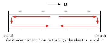
vaft.diagram.blob_current_closure(regime='sheath')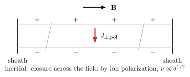
vaft.diagram.blob_current_closure(regime='inertial')Where the polarization current of a filament closes: the sheaths or the cross-field inertia.
vaft.diagram.blob_current_closure(*, regime='sheath', labels=True)Show source vaft/diagram/_blob.py, lines 111–157
def blob_current_closure(*, regime: str = "sheath", labels: bool = True) -> Diagram:
r"""Where the polarization current of a filament closes: the sheaths or the cross-field inertia.
The filament drawn along $\mathbf B$ between two targets, its dipole as
a charge excess along the top and a deficit along the bottom.
``regime="sheath"``: the current runs along the field to both sheaths
and returns through them -- the least resistive path, the lowest
potential and speed, $v \propto \delta^{-2}$. ``"inertial"``: the
filament is cut off from the sheaths (by resistivity or X-point
fanning) and the current closes across the field by the ion
polarization current near the midplane, $v \propto \delta^{1/2}$.
"""
labels = _check_labels(labels)
if regime not in ("sheath", "inertial"):
raise ValueError(f"regime must be 'sheath' or 'inertial', not {regime!r}")
L, h = 8.0, 1.2
items: List = [Polyline.of([(0.0, -0.3), (0.0, h + 0.3)], "machine", role="sheath_left"),
Polyline.of([(L, -0.3), (L, h + 0.3)], "machine", role="sheath_right"),
Polyline.of([(0.0, h), (L, h)], "surface", role="filament"),
Polyline.of([(0.0, 0.0), (L, 0.0)], "surface", role="filament"),
Arrow((L / 2 - 0.6, h + 0.9), (L / 2 + 0.6, h + 0.9), "vector", role="magnetic_field")]
for x in np.linspace(1.0, L - 1.0, 4):
items += [Label((float(x), h + 0.25), "$+$", "small label", role="charge_positive"),
Label((float(x), -0.25), "$-$", "small label", role="charge_negative")]
if regime == "sheath":
# along the top to each sheath, down through it, back along the bottom
for side in (-1.0, 1.0):
x0, x1 = L / 2 + side * 0.4, (L if side > 0 else 0.0) - side * 0.25
items += [Arrow((x0, h - 0.2), (x1, h - 0.2), "drift", role="parallel_current"),
Arrow((x1, h - 0.3), (x1, 0.3), "drift", role="sheath_current"),
Arrow((x1, 0.2), (x0, 0.2), "drift", role="parallel_current")]
else:
# cut off from the sheaths; closure across the field at the midplane by ion polarization
for x in (1.6, L - 1.6):
items.append(Polyline.of([(x - 0.15, -0.1), (x + 0.15, h + 0.1)], "leader line", role="disconnection"))
items.append(Arrow((L / 2, h - 0.2), (L / 2, 0.2), "drift", role="polarization_current"))
if labels:
title = {"sheath": "sheath-connected: closure through the sheaths, $v \\propto \\delta^{-2}$",
"inertial": "inertial: closure across the field by ion polarization, $v \\propto \\delta^{1/2}$"}
items += [Label((L / 2 + 0.7, h + 0.9), "$\\mathbf B$", "small label", anchor="west", role="magnetic_field"),
Label((0.0, -0.4), "sheath", "small label", anchor="north", role="sheath_left"),
Label((L, -0.4), "sheath", "small label", anchor="north", role="sheath_right"),
Label((L / 2, -0.75), title[regime], "small label", anchor="north", role="title")]
if regime == "inertial":
items.append(Label((L / 2 + 0.15, h / 2), "$J_{\\perp,\\mathrm{pol}}$", "small label", anchor="west",
role="polarization_current"))
return Diagram("blob_current_closure", Scene(tuple(items)), model={"regime": regime})Formats .svg .tex .pdf the SVG above is committed; build the others locally
import vaft.diagram
d = vaft.diagram.blob_current_closure(regime='sheath')
d.tikz # the TikZ document as text
d.save("blob_current_closure_sheath.svg") # rendered vector image, the canonical artifact; needs latex, dvisvgm
d.save("blob_current_closure_sheath.tex") # the complete TikZ document, the text source
d.save("blob_current_closure_sheath.pdf") # vector PDF; needs pdflatexblob_velocity_scaling
1 asset
source
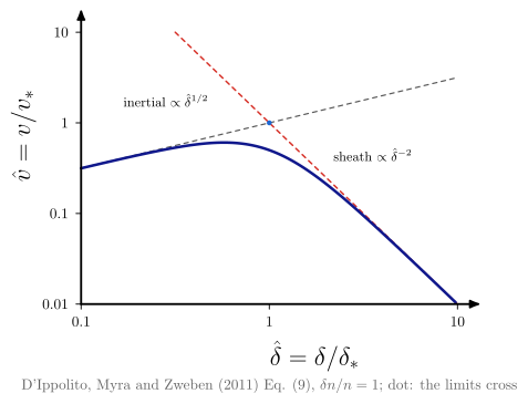
vaft.diagram.blob_velocity_scaling()Normalized blob velocity against normalized size: two closures, their crossing, and the bridge.
vaft.diagram.blob_velocity_scaling(*, relative_amplitude=1.0, labels=True)Show source vaft/diagram/_blob.py, lines 160–195
def blob_velocity_scaling(*, relative_amplitude: float = 1.0, labels: bool = True) -> Diagram:
r"""Normalized blob velocity against normalized size: two closures, their crossing, and the bridge.
Log--log $\hat v = v/v_*$ against $\hat\delta = \delta/\delta_*$ with the
inertial limit $(\delta n/n)^{1/2}\hat\delta^{1/2}$ (current closed across
the field), the sheath-connected limit $(\delta n/n)/\hat\delta^2$ (closed
at the sheaths), their crossing at ``blob_crossover_size``, and
``interpolated_blob_velocity``, which peaks at $0.574$ of the crossing.
"""
labels = _check_labels(labels)
ld = np.linspace(-1.0, 1.0, 201)
d = 10.0**ld
f = float(relative_amplitude)
v = np.asarray(interpolated_blob_velocity(d, relative_amplitude=f))
inertial, sheath = np.sqrt(f) * np.sqrt(d), f / d**2
dc = float(blob_crossover_size(relative_amplitude=f))
chart = Chart(x_range=(-1.0, 1.0), y_range=(-2.0, 1.0))
chart.curves.update({"interpolated": np.stack([ld, np.log10(v)], -1),
"inertial": np.stack([ld, np.log10(inertial)], -1),
"sheath": np.stack([ld, np.log10(sheath)], -1)})
chart.points["crossover"] = (math.log10(dc), math.log10(math.sqrt(f) * math.sqrt(dc)))
chart.labels.update({"inertial": (-0.55, 0.25), "sheath": (0.55, -0.35)})
chart.parameters.update({"relative_amplitude": f, "crossover": dc})
scene = render_chart(
chart, x_label="$\\hat\\delta = \\delta/\\delta_*$", y_label="$\\hat v = v/v_*$",
curve_styles={"inertial": "approx", "sheath": "slope plus", "interpolated": "boundary"},
region_text={"inertial": "\\small inertial $\\propto\\hat\\delta^{1/2}$",
"sheath": "\\small sheath $\\propto\\hat\\delta^{-2}$"} if labels else {},
x_ticks=[-1.0, 0.0, 1.0], x_tick_text=["$0.1$", "$1$", "$10$"], y_ticks=[-2.0, -1.0, 0.0, 1.0],
y_tick_text=["$0.01$", "$0.1$", "$1$", "$10$"],
note=(f"D'Ippolito, Myra and Zweben (2011) Eq. (9), $\\delta n/n = {f:g}$; dot: the limits cross" if labels
else ""),
)
items = list(scene.items) + [Marker(tuple(chart.to_cm(np.array(chart.points["crossover"]))), "o", "opoint",
role="crossover")]
return Diagram("blob_velocity_scaling", Scene(tuple(items)), model=chart)Formats .svg .tex .pdf the SVG above is committed; build the others locally
import vaft.diagram
d = vaft.diagram.blob_velocity_scaling()
d.tikz # the TikZ document as text
d.save("blob_velocity_scaling.svg") # rendered vector image, the canonical artifact; needs latex, dvisvgm
d.save("blob_velocity_scaling.tex") # the complete TikZ document, the text source
d.save("blob_velocity_scaling.pdf") # vector PDF; needs pdflatexFormula functions referenced:
sol.blob_crossover_size, sol.interpolated_blob_velocity
blob_regimes
1 asset
source
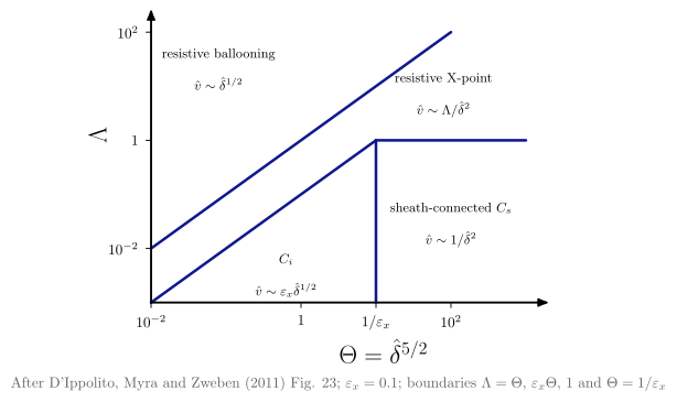
vaft.diagram.blob_regimes()The two-region regime plane of blob motion: collisionality against size.
vaft.diagram.blob_regimes(*, epsilon_x=0.1, labels=True)Show source vaft/diagram/_blob.py, lines 198–251
def blob_regimes(*, epsilon_x: float = EPSILON_X, labels: bool = True) -> Diagram:
r"""The two-region regime plane of blob motion: collisionality against size.
$\log\Lambda$ against $\log\Theta$, $\Theta = \hat\delta^{5/2}$. The
boundaries are where neighbouring scalings of ``blob_regime_velocities``
are equal -- $\Lambda = \Theta$, $\Lambda = \varepsilon_x\Theta$,
$\Lambda = 1$ and $\Theta = 1/\varepsilon_x$ -- around resistive ballooning
(RB, upper left), resistive X-point (RX, the middle band), connected
ideal interchange ($C_i$, lower left) and sheath-connected ($C_s$, lower
right). ``epsilon_x`` is the X-point fanning, ~0.1 at 1 cm into the SOL.
"""
labels = _check_labels(labels)
if not 0.0 < epsilon_x < 1.0:
raise ValueError(f"epsilon_x must lie in (0, 1), not {epsilon_x!r}")
le = math.log10(1.0 / epsilon_x) # log of the Theta where C_i meets C_s
x0, x1 = -2.0, max(3.0, le + 1.5)
lt = np.linspace(x0, x1, 251)
theta = 10.0**lt
d = theta**0.4
v = blob_regime_velocities(d, 1.0, epsilon_x)
# each boundary: the Lambda at which two scalings are equal (RX is linear in Lambda)
rb_rx = np.asarray(v.resistive_ballooning) / np.asarray(v.resistive_x_point)
rx_ci = np.asarray(v.connected_ideal_interchange) / np.asarray(v.resistive_x_point)
y0, y1 = -3.0, 2.0
chart = Chart(x_range=(x0, x1), y_range=(y0, y1))
chart.curves.update({
"rb_rx": np.stack([lt, np.log10(rb_rx)], -1),
"rx_ci": np.stack([lt[lt <= le], np.log10(rx_ci[lt <= le])], -1),
"rx_cs": np.array([[le, 0.0], [x1, 0.0]]),
"ci_cs": np.array([[le, y0], [le, 0.0]]),
})
# regions placed relative to the boundaries, so they move with epsilon_x
chart.labels.update({"RB": (x0 + 0.3 * (le - x0), 1.35), "RX": (le + 0.9, 0.9),
"Ci": (x0 + 0.6 * (le - x0), -2.45), "Cs": (le + 0.5 * (x1 - le), -1.5)})
chart.parameters.update({"epsilon_x": epsilon_x, "theta_ci_cs": 1.0 / epsilon_x})
ticks = sorted({-2.0, 0.0, 2.0} | {round(le, 6)})
tick_text = [("$1/\\varepsilon_x$" if abs(t - le) < 1e-9 else f"$10^{{{int(t)}}}$" if t else "$1$") for t in ticks]
scene = render_chart(
chart, x_label="$\\Theta = \\hat\\delta^{5/2}$", y_label="$\\Lambda$",
curve_styles={"rb_rx": "boundary", "rx_ci": "boundary", "rx_cs": "boundary", "ci_cs": "boundary"},
region_text={"RB": "\\begin{tabular}{c}\\small resistive ballooning\\\\\\small $\\hat v\\sim\\hat\\delta^{1/2}$"
"\\end{tabular}",
"RX": "\\begin{tabular}{c}\\small resistive X-point\\\\\\small $\\hat v\\sim\\Lambda/\\hat\\delta^2$"
"\\end{tabular}",
"Ci": "\\begin{tabular}{c}\\small $C_i$\\\\\\small $\\hat v\\sim\\varepsilon_x\\hat\\delta^{1/2}$"
"\\end{tabular}",
"Cs": "\\begin{tabular}{c}\\small sheath-connected $C_s$\\\\\\small $\\hat v\\sim 1/\\hat\\delta^2$"
"\\end{tabular}"} if labels else {},
x_ticks=ticks, x_tick_text=tick_text,
y_ticks=[-2.0, 0.0, 2.0], y_tick_text=["$10^{-2}$", "$1$", "$10^{2}$"],
note=(f"After D'Ippolito, Myra and Zweben (2011) Fig. 23; $\\varepsilon_x = {epsilon_x:g}$; boundaries "
"$\\Lambda = \\Theta$, $\\varepsilon_x\\Theta$, $1$ and $\\Theta = 1/\\varepsilon_x$" if labels else ""),
)
return Diagram("blob_regimes", scene, model=chart)Formats .svg .tex .pdf the SVG above is committed; build the others locally
import vaft.diagram
d = vaft.diagram.blob_regimes()
d.tikz # the TikZ document as text
d.save("blob_regimes.svg") # rendered vector image, the canonical artifact; needs latex, dvisvgm
d.save("blob_regimes.tex") # the complete TikZ document, the text source
d.save("blob_regimes.pdf") # vector PDF; needs pdflatexFormula functions referenced:
sol.blob_regime_velocities
MARFE: a localized radiation condensation on an equilibrium, and the condition that makes it
Module vaft.diagram._marfe
marfe
2 assets
source
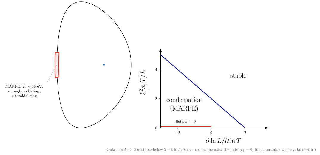
vaft.diagram.marfe()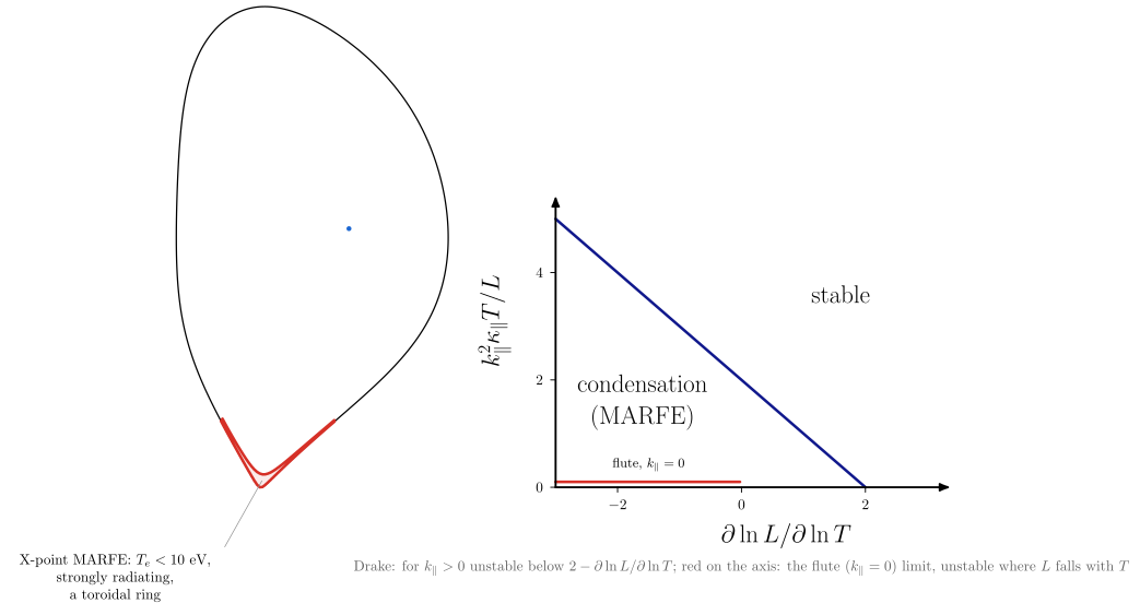
vaft.diagram.marfe(localization='xpoint')A MARFE on the edge of an equilibrium, and Drake’s condensation condition.
vaft.diagram.marfe(equilibrium=None, *, localization='hfs', poloidal_width_deg=30.0, radial_fraction=0.1, labels=True)Show source vaft/diagram/_marfe.py, lines 154–219
def marfe(equilibrium=None, *, localization: str = "hfs", poloidal_width_deg: float = POLOIDAL_WIDTH_DEG,
radial_fraction: float = RADIAL_FRACTION, labels: bool = True) -> Diagram:
r"""A MARFE on the edge of an equilibrium, and Drake's condensation condition.
Left: a prescribed radiating band. On the high-field side
(``localization="hfs"``) it straddles the last closed surface, ~30
degrees wide and ~10 % of $a$ deep (Lipschultz 1987); next to the X-point
(``"xpoint"``, Greenwald 2002 p. R35) it sits on the closed side with the
same borrowed sizes. Its $T_e$ is below ~10 eV (Greenwald p. R34); the
density rise at constant pressure is Drake's model (his Eq. 17); it is
toroidally symmetric, a ring. Right: the plane of radiation slope
$\partial\ln L/\partial\ln T$ and conduction ratio
$k_\parallel^2\kappa_\parallel T/L$, with the condensation boundary where
``radiative_condensation_growth_rate`` vanishes; on the $k_\parallel = 0$
axis, where the flute limit applies, the segment on which
``radiative_thermal_instability_growth_rate`` is positive.
"""
labels = _check_labels(labels)
m = marfe_region(equilibrium, localization=localization, poloidal_width_deg=poloidal_width_deg,
radial_fraction=radial_fraction)
lcfs, axis = m["lcfs"], np.asarray(m["axis"])
ox, oy = -_SCALE * float(np.min(lcfs[:, 0])) + 0.6, -_SCALE * float(np.min(lcfs[:, 1])) + 0.4
def cm(pts):
pts = np.asarray(pts, dtype=float)
return np.stack([_SCALE * pts[..., 0] + ox, _SCALE * pts[..., 1] + oy], -1)
items: List = [Polyline.of(cm(lcfs), "lcfs", role="lcfs", closed=True),
Polyline.of(cm(m["outline"]), "layer", role="marfe", closed=True),
Polyline.of(cm(m["outline"]), "inner solution", role="marfe_edge", closed=True),
Marker(tuple(cm(axis)), "o", "opoint", role="magnetic_axis")]
left_width = float(cm([np.max(lcfs[:, 0]), 0.0])[0]) + 0.6
if labels:
c = cm(m["centre_point"])
side = -1.0 if math.cos(m["centre_angle"]) < 0 else 1.0
# outside the plasma, on the MARFE's own side, so the label never covers the boundary
tip = (float(c[0]) + side * 0.9, float(c[1]) - 1.6)
name = "MARFE" if localization == "hfs" else "X-point MARFE"
items += [Polyline.of([tuple(c), tip], "leader line", role="marfe"),
Label(tip, f"\\begin{{tabular}}{{c}}{name}: $T_e < 10$ eV,\\\\ strongly radiating,\\\\"
" a toroidal ring\\end{tabular}", "small label",
anchor="north east" if side < 0 else "north west", role="marfe")]
# right: the condensation plane (k_parallel > 0) and the flute limit on its k_parallel = 0 axis
x = np.linspace(-3.0, 3.0, 241)
y_marg = condensation_boundary(x)
chart = Chart(x_range=(-3.0, 3.0), y_range=(0.0, 5.0))
chart.curves["condensation"] = np.stack([x, y_marg], -1)
# the flute growth rate at slope x (any L/T > 0): unstable where it is positive
flute_growth = np.array([radiative_thermal_instability_growth_rate(1e19, xi * 1e5 / 5.0) for xi in x])
# drawn just above the k_parallel = 0 axis so the axis line does not hide it
chart.curves["flute"] = np.stack([x[flute_growth > 0], np.full(int(np.sum(flute_growth > 0)), 0.1)], -1)
chart.labels.update({"stable": (1.6, 3.6), "unstable": (-1.6, 1.6), "flute": (-1.5, 0.42)})
chart.parameters.update({"poloidal_width_deg": m["poloidal_width_deg"], "radial_fraction": m["radial_fraction"]})
scene = render_chart(
chart, x_label="$\\partial\\ln L/\\partial\\ln T$", y_label="$k_\\parallel^2\\kappa_\\parallel T/L$",
curve_styles={"condensation": "boundary", "flute": "inner solution"},
region_text={"stable": "stable", "unstable": "\\begin{tabular}{c}condensation\\\\(MARFE)\\end{tabular}",
"flute": "\\small flute, $k_\\parallel = 0$"} if labels else {},
x_ticks=[-2.0, 0.0, 2.0], y_ticks=[0.0, 2.0, 4.0],
note=("Drake: for $k_\\parallel > 0$ unstable below $2 - \\partial\\ln L/\\partial\\ln T$; red on the axis: "
"the flute ($k_\\parallel = 0$) limit, unstable where $L$ falls with $T$" if labels else ""),
)
items += list(scene.transformed(offset=(left_width + 2.0, 0.4)).items)
model = {k: v for k, v in m.items() if k != "equilibrium"}
model["chart"] = chart
return Diagram("marfe", Scene(tuple(items)), model=model)Formats .svg .tex .pdf the SVG above is committed; build the others locally
import vaft.diagram
d = vaft.diagram.marfe()
d.tikz # the TikZ document as text
d.save("marfe.svg") # rendered vector image, the canonical artifact; needs latex, dvisvgm
d.save("marfe.tex") # the complete TikZ document, the text source
d.save("marfe.pdf") # vector PDF; needs pdflatexFormula functions referenced:
sol.radiative_condensation_growth_rate, sol.radiative_thermal_instability_growth_rate
Divertor heat-flux footprint: an Eich target profile mapped onto a diverted equilibrium
Module vaft.diagram._divertor_footprint
divertor_heat_footprint
1 asset
source
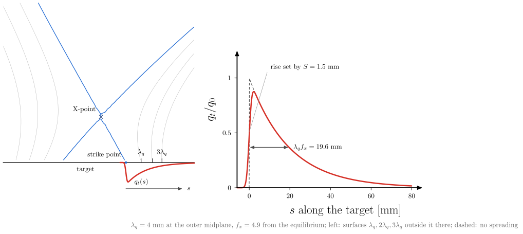
vaft.diagram.divertor_heat_footprint()An Eich heat-flux profile on the divertor target of a diverted equilibrium.
vaft.diagram.divertor_heat_footprint(equilibrium=None, *, lambda_q=0.004, spreading=0.0015, target='outer', target_z=None, labels=True)Formats .svg .tex .pdf the SVG above is committed; build the others locally
import vaft.diagram
d = vaft.diagram.divertor_heat_footprint()
d.tikz # the TikZ document as text
d.save("divertor_heat_footprint.svg") # rendered vector image, the canonical artifact; needs latex, dvisvgm
d.save("divertor_heat_footprint.tex") # the complete TikZ document, the text source
d.save("divertor_heat_footprint.pdf") # vector PDF; needs pdflatexFormula functions referenced:
sol.eich_integral_width, sol.eich_target_heat_flux_profile
Integrated-modeling diagrams: three independent model axes, their space, and model coupling
Module vaft.diagram._integrated_modeling
knowledge_basis
1 asset
source
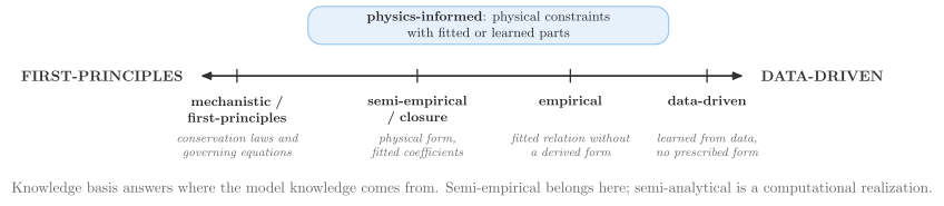
vaft.diagram.knowledge_basis()Where a model’s knowledge comes from: first-principles to data-driven.
vaft.diagram.knowledge_basis(*, labels=True)Show source vaft/diagram/_integrated_modeling.py, lines 60–96
def knowledge_basis(*, labels: bool = True) -> Diagram:
r"""Where a model's knowledge comes from: first-principles to data-driven.
Four stations on one axis -- mechanistic/first-principles,
semi-empirical/closure, empirical, data-driven -- each with a generic
example. Physics-informed models combine physical constraints with
fitted or learned parts, so they are drawn as a bridge spanning the axis,
not as a point on it. Semi-empirical is a knowledge basis;
semi-analytical is a computational realization (``computational_realization``).
"""
labels = _check_labels(labels)
width = 13.0
items: List = [Arrow((0.0, 0.0), (width, 0.0), "im axis", role="axis", both=True)]
lo, hi = schema.PHYSICS_INFORMED_SPAN
items.append(Polyline.of([(lo * width, 0.75), (hi * width, 0.75), (hi * width, 1.65), (lo * width, 1.65)],
"im bridge", role="knowledge:physics_informed", closed=True))
items.append(Label((0.5 * (lo + hi) * width, 1.2),
"\\textbf{physics-informed}: physical constraints\\\\ with fitted or learned parts",
"im station", role="knowledge:physics_informed"))
for key, text, pos, example in schema.KNOWLEDGE_BASIS:
x = pos * width
items += [Polyline.of([(x, -0.15), (x, 0.15)], "im tick", role=f"knowledge:{key}"),
Label((x, -0.35), f"\\textbf{{{text}}}", "im station,text width=3.6cm", anchor="north",
role=f"knowledge:{key}")]
if labels:
items.append(Label((x, -1.25), example, "im example,text width=3.6cm", anchor="north",
role=f"knowledge:{key}:example"))
items += [Label((-0.25, 0.0), "FIRST-PRINCIPLES", "im axis title", anchor="east", role="axis"),
Label((width + 0.25, 0.0), "DATA-DRIVEN", "im axis title", anchor="west", role="axis")]
if labels:
items.append(Label((0.5 * width, -2.4), "Knowledge basis answers where the model knowledge comes from. "
"Semi-empirical belongs here; semi-analytical is a computational realization.",
"note", anchor="north", role="note"))
model = {"axis": ("first-principles", "data-driven"),
"stations": tuple(k for k, *_ in schema.KNOWLEDGE_BASIS),
"bridge": ("physics_informed", schema.PHYSICS_INFORMED_SPAN)}
return Diagram("knowledge_basis", Scene(tuple(items)), model=model)Formats .svg .tex .pdf the SVG above is committed; build the others locally
import vaft.diagram
d = vaft.diagram.knowledge_basis()
d.tikz # the TikZ document as text
d.save("knowledge_basis.svg") # rendered vector image, the canonical artifact; needs latex, dvisvgm
d.save("knowledge_basis.tex") # the complete TikZ document, the text source
d.save("knowledge_basis.pdf") # vector PDF; needs pdflatexcomputational_realization
1 asset
source
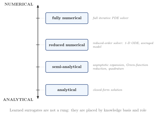
vaft.diagram.computational_realization()How a model is evaluated: analytical, semi-analytical, reduced numerical, fully numerical.
vaft.diagram.computational_realization(*, labels=True)Show source vaft/diagram/_integrated_modeling.py, lines 99–126
def computational_realization(*, labels: bool = True) -> Diagram:
r"""How a model is evaluated: analytical, semi-analytical, reduced numerical, fully numerical.
A ladder from the closed form at the bottom to the full iterative PDE
solver at the top, each rung with generic examples. Learned surrogates
and neural operators are not a rung: they are placed in the modeling
space by their knowledge basis and their role.
"""
labels = _check_labels(labels)
height, box_w, box_h = 8.0, 3.8, 1.0
items: List = [Arrow((0.0, -0.3), (0.0, height + 0.3), "im axis", role="axis", both=True)]
for key, text, pos, example in schema.COMPUTATIONAL_REALIZATION:
y = pos * height
b = box(2.6, y, box_w, box_h, f"\\textbf{{{text}}}", role=f"realization:{key}", latex=True)
items += [Polyline.of([(-0.15, y), (0.15, y)], "im tick", role=f"realization:{key}"),
Polyline.of([(0.15, y), (2.6 - 0.5 * box_w, y)], "im grid", role=f"realization:{key}")]
items += list(b.items)
if labels:
items.append(Label((2.6 + 0.5 * box_w + 0.3, y), example, "im example,text width=5.6cm,align=left",
anchor="west", role=f"realization:{key}:example"))
items += [Label((-0.3, -0.3), "ANALYTICAL", "im axis title", anchor="east", role="axis"),
Label((-0.3, height + 0.3), "NUMERICAL", "im axis title", anchor="east", role="axis")]
if labels:
items.append(Label((3.6, -1.0), "Learned surrogates are not a rung: they are placed by knowledge basis "
"and role", "note", anchor="north", role="note"))
model = {"axis": ("analytical", "numerical"),
"rungs": tuple(k for k, *_ in schema.COMPUTATIONAL_REALIZATION)}
return Diagram("computational_realization", Scene(tuple(items)), model=model)Formats .svg .tex .pdf the SVG above is committed; build the others locally
import vaft.diagram
d = vaft.diagram.computational_realization()
d.tikz # the TikZ document as text
d.save("computational_realization.svg") # rendered vector image, the canonical artifact; needs latex, dvisvgm
d.save("computational_realization.tex") # the complete TikZ document, the text source
d.save("computational_realization.pdf") # vector PDF; needs pdflatexphysical_abstraction
1 asset
source
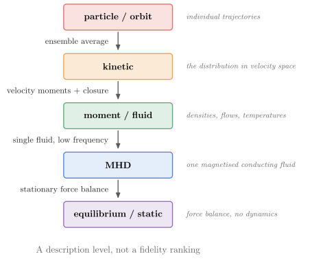
vaft.diagram.physical_abstraction()At what description level the system is represented, and how each level reduces to the next.
vaft.diagram.physical_abstraction(*, labels=True)Show source vaft/diagram/_integrated_modeling.py, lines 129–159
def physical_abstraction(*, labels: bool = True) -> Diagram:
r"""At what description level the system is represented, and how each level reduces to the next.
Particle/orbit, kinetic, moment/fluid, MHD, equilibrium/static, each
with what it resolves; the arrows are the reductions -- ensemble average,
velocity moments with a closure, single fluid at low frequency,
stationary force balance. A description level, not a fidelity ranking:
each level is adequate for the questions it keeps.
"""
labels = _check_labels(labels)
step, box_w, box_h = 1.9, 4.2, 1.0
items: List = []
levels: List[Box] = []
for i, (key, text, resolves) in enumerate(schema.PHYSICAL_ABSTRACTION):
y = -i * step
b = box(0.0, y, box_w, box_h, f"\\textbf{{{text}}}", style=f"im level {key}", role=f"abstraction:{key}",
latex=True)
levels.append(b)
items += list(b.items)
if labels:
items.append(Label((0.5 * box_w + 0.4, y), resolves, "im example,text width=4.6cm,align=left",
anchor="west", role=f"abstraction:{key}:resolves"))
for (a, b), reduction in zip(zip(levels, levels[1:]), schema.ABSTRACTION_REDUCTIONS):
items.append(connector(a, b, style="im reduction", role="abstraction:reduction"))
items.append(Label((-0.25, 0.5 * (a.y + b.y)), reduction, "im station", anchor="east",
role="abstraction:reduction"))
if labels:
items.append(Label((0.0, -(len(levels) - 1) * step - 1.1),
"A description level, not a fidelity ranking", "note", anchor="north", role="note"))
model = {"levels": _ABSTRACTION_KEYS, "reductions": schema.ABSTRACTION_REDUCTIONS}
return Diagram("physical_abstraction", Scene(tuple(items)), model=model)Formats .svg .tex .pdf the SVG above is committed; build the others locally
import vaft.diagram
d = vaft.diagram.physical_abstraction()
d.tikz # the TikZ document as text
d.save("physical_abstraction.svg") # rendered vector image, the canonical artifact; needs latex, dvisvgm
d.save("physical_abstraction.tex") # the complete TikZ document, the text source
d.save("physical_abstraction.pdf") # vector PDF; needs pdflatexintegrated_modeling_space
3 assets
source
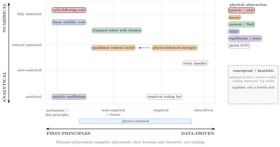
vaft.diagram.integrated_modeling_space()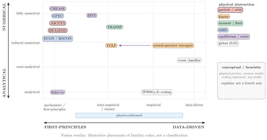
vaft.diagram.integrated_modeling_space(examples='fusion')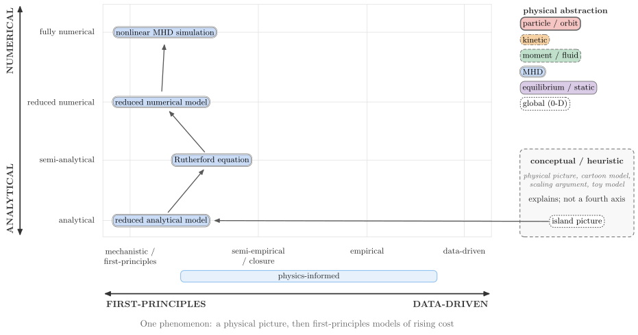
vaft.diagram.integrated_modeling_space(examples='tearing')The three axes combined: where models sit, and what character they have.
vaft.diagram.integrated_modeling_space(examples='generic', *, labels=True)Formats .svg .tex .pdf the SVG above is committed; build the others locally
import vaft.diagram
d = vaft.diagram.integrated_modeling_space()
d.tikz # the TikZ document as text
d.save("integrated_modeling_space.svg") # rendered vector image, the canonical artifact; needs latex, dvisvgm
d.save("integrated_modeling_space.tex") # the complete TikZ document, the text source
d.save("integrated_modeling_space.pdf") # vector PDF; needs pdflatexintegrated_modeling_process
1 asset
source
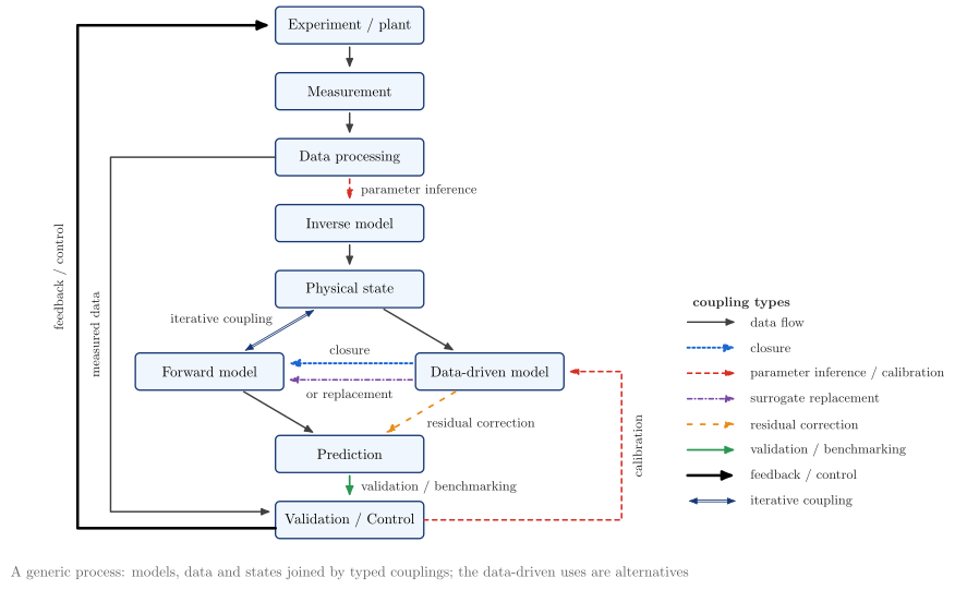
vaft.diagram.integrated_modeling_process()How models interact: a graph of models, data and states with typed couplings.
vaft.diagram.integrated_modeling_process(*, labels=True)Show source vaft/diagram/_integrated_modeling.py, lines 276–353
def integrated_modeling_process(*, labels: bool = True) -> Diagram:
r"""How models interact: a graph of models, data and states with typed couplings.
The experiment is measured; processed data feed an inverse model --
parameter inference -- that yields a physical state. A forward model,
coupled iteratively to that state, gives a prediction. A data-driven
model is used in one of several alternative ways: as a closure inside
the forward model, or as its surrogate replacement, or as a residual
correction of its prediction (the hybrid mode). Validation compares the
prediction with the processed measurement, calibrates the data-driven
model and closes the loop as feedback or control on the experiment. The
legend lists the coupling types; a coupling is a label on an edge.
"""
labels = _check_labels(labels)
items: List = []
nodes: Dict[str, Box] = {}
for role, text in schema.PROCESS_NODES:
x, y = _PROCESS_AT[role]
b = box(x, y, _NODE_W, _NODE_H, text, role=f"node:{role}")
nodes[role] = b
items += list(b.items)
hw, gap = 0.5 * _NODE_W, 0.08
for c in schema.PROCESS_COUPLINGS:
style, role = _coupling_style(c.coupling), f"coupling:{c.coupling}"
s, t = nodes[c.source], nodes[c.target]
if c.coupling == "feedback": # around the far left, up to the experiment
x, y0 = -6.6, s.y - 0.2
items.append(Polyline.of([(s.x - hw, y0), (x, y0), (x, t.y), (t.x - hw - gap, t.y)], style, role=role))
if labels:
items.append(Label((x - 0.15, 0.5 * (y0 + t.y)), "feedback / control", "im station,rotate=90",
anchor="south", role=role))
elif c.source == "processing" and c.target == "validation": # the measured data validation compares with
x, y1 = -5.8, t.y + 0.2
items.append(Polyline.of([(s.x - hw, s.y), (x, s.y), (x, y1), (t.x - hw - gap, y1)], style, role=role))
if labels:
items.append(Label((x - 0.15, 0.5 * (s.y + y1)), "measured data", "im station,rotate=90",
anchor="south", role=role))
elif c.source == "validation" and c.target == "data_driven": # around the right, up into the model
x = 6.6
items.append(Polyline.of([(s.x + hw, s.y), (x, s.y), (x, t.y), (t.x + hw + gap, t.y)], style,
role=role))
if labels:
items.append(Label((x + 0.15, 0.5 * (s.y + t.y)), "calibration", "im station,rotate=90",
anchor="north", role=role))
elif c.source == "data_driven" and c.target == "forward": # alternative uses of one data-driven model
dy = 0.2 if c.coupling == "closure" else -0.2
items.append(Arrow((s.x - hw - gap, s.y + dy), (t.x + hw + gap, t.y + dy), style, role=role))
if labels:
text = "closure" if c.coupling == "closure" else "or replacement"
items.append(Label((0.0, s.y + dy + (0.1 if dy > 0 else -0.1)), text, "im station",
anchor="south" if dy > 0 else "north", role=role))
else:
arrow = connector(s, t, style=style, role=role)
if c.coupling == "iterative":
arrow = Arrow(arrow.start, arrow.end, style, role=role, both=True)
items.append(arrow)
if labels and c.coupling in ("iterative", "residual", "validation", "calibration"):
mid = 0.5 * (np.asarray(arrow.start) + np.asarray(arrow.end))
text = {"calibration": "parameter inference"}.get(c.coupling, _COUPLING_LABEL[c.coupling])
if abs(arrow.end[0] - arrow.start[0]) < 1e-9: # vertical: beside it
items.append(Label((mid[0] + 0.15, mid[1]), text, "im station", anchor="west", role=role))
else: # diagonal: just outside its outer side
side = "south east" if mid[0] < 0.0 else "north west"
items.append(Label((mid[0] + (-0.05 if mid[0] < 0 else 0.05), mid[1]), text, "im station",
anchor=side, role=role))
# legend of every coupling type, bottom right
lx, ly = 8.2, 3.6
items.append(Label((lx, ly + 0.2), "\\textbf{coupling types}", "im station", anchor="south west", role="legend"))
for i, (key, text) in enumerate(schema.COUPLING_TYPES):
y = ly - 0.62 * i
items += [Arrow((lx, y), (lx + 1.2, y), _coupling_style(key), role=f"legend:{key}", both=key == "iterative"),
Label((lx + 1.4, y), text, "im station", anchor="west", role=f"legend:{key}")]
if labels:
items.append(Label((0.0, -2.2), "A generic process: models, data and states joined by typed couplings; "
"the data-driven uses are alternatives", "note", anchor="north", role="note"))
model = {"nodes": tuple(r for r, _ in schema.PROCESS_NODES), "couplings": schema.PROCESS_COUPLINGS,
"coupling_types": tuple(k for k, _ in schema.COUPLING_TYPES)}
return Diagram("integrated_modeling_process", Scene(tuple(items)), model=model)Formats .svg .tex .pdf the SVG above is committed; build the others locally
import vaft.diagram
d = vaft.diagram.integrated_modeling_process()
d.tikz # the TikZ document as text
d.save("integrated_modeling_process.svg") # rendered vector image, the canonical artifact; needs latex, dvisvgm
d.save("integrated_modeling_process.tex") # the complete TikZ document, the text source
d.save("integrated_modeling_process.pdf") # vector PDF; needs pdflatexVAFT framework concept diagrams (#1090): what the framework is and how scientific data moves through it
Module vaft.diagram._vaft_concepts
fusion_science_knowledge_lifecycle
1 asset
source
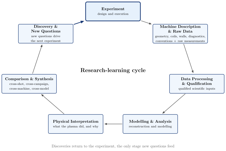
vaft.diagram.fusion_science_knowledge_lifecycle()The research-learning cycle the infrastructure enables: from experiment back to experiment.
vaft.diagram.fusion_science_knowledge_lifecycle(*, labels=True)Show source vaft/diagram/_vaft_concepts.py, lines 188–225
def fusion_science_knowledge_lifecycle(*, labels: bool = True) -> Diagram:
r"""The research-learning cycle the infrastructure enables: from experiment back to experiment.
Experiment; machine description and raw data -- the computationally
usable machine (geometry, coils, walls, diagnostics, configurations,
conventions) together with the raw measurements, kept apart from later
plasma modelling; data processing and qualification into qualified
scientific inputs (verification and validation cut across the whole
pipeline, ``scientific_workflow``); modelling and analysis; physical
interpretation; comparison and synthesis across shots, campaigns,
machines and models; and discovery and new
questions, which feed back into the design and execution of the next
experiment -- the only stage they return to.
"""
labels = _check_labels(labels)
items: List = []
edges: List = []
boxes: Dict[str, Box] = {}
rx, ry, w, h = 7.7, 5.3, 4.9, 1.7
n = len(LIFECYCLE)
for i, (key, title, sub) in enumerate(LIFECYCLE):
a = math.radians(90.0 - 360.0 * i / n)
style = "concept strong" if key == "experiment" else "concept box"
b = box(rx * math.cos(a), ry * math.sin(a), w, h, _titled(title, sub, sub_size="footnotesize"), style=style,
role=f"node:{key}", latex=True)
boxes[key] = b
items += list(b.items)
keys = [k for k, _, _ in LIFECYCLE]
for k0, k1 in zip(keys, keys[1:]):
_edge(items, edges, boxes[k0], boxes[k1], k0, k1)
# discoveries drive the next experiment: the one feedback edge, drawn stronger
_edge(items, edges, boxes["discovery"], boxes["experiment"], "discovery", "experiment", style="connector strong")
items.append(Label((0.0, 0.0), "{\\Large\\textbf{Research-learning cycle}}", "concept plain", role="title"))
if labels:
items.append(Label((0.0, -ry - 1.2), "Discoveries return to the experiment, the only stage new questions feed",
"note", anchor="north", role="note"))
return Diagram("fusion_science_knowledge_lifecycle", Scene(tuple(items)),
model={"nodes": tuple(keys), "edges": tuple(edges), "feedback": ("discovery", "experiment")})Formats .svg .tex .pdf the SVG above is committed; build the others locally
import vaft.diagram
d = vaft.diagram.fusion_science_knowledge_lifecycle()
d.tikz # the TikZ document as text
d.save("fusion_science_knowledge_lifecycle.svg") # rendered vector image, the canonical artifact; needs latex, dvisvgm
d.save("fusion_science_knowledge_lifecycle.tex") # the complete TikZ document, the text source
d.save("fusion_science_knowledge_lifecycle.pdf") # vector PDF; needs pdflatexvaft_four_pillars
1 asset
source
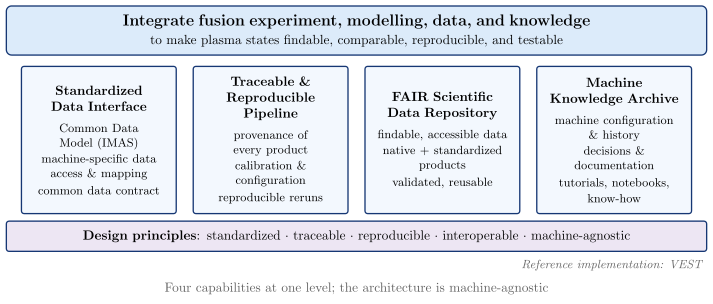
vaft.diagram.vaft_four_pillars()The four pillars of VAFT, under its purpose and on its design principles.
vaft.diagram.vaft_four_pillars(*, labels=True)Show source vaft/diagram/_vaft_concepts.py, lines 134–173
def vaft_four_pillars(*, labels: bool = True) -> Diagram:
r"""The four pillars of VAFT, under its purpose and on its design principles.
An architecture figure: four capabilities at one level of abstraction --
a standardized data interface, a traceable and reproducible pipeline, a
FAIR scientific data repository and a machine knowledge archive -- hold
up the purpose: integrate fusion experiment, modelling, data and
knowledge so that plasma states are findable, comparable, reproducible
and testable. They stand on the shared design principles. The research
process they serve is ``fusion_science_knowledge_lifecycle``. VEST is
labelled as the reference implementation, not drawn as the foundation:
the architecture is machine-agnostic.
"""
labels = _check_labels(labels)
width, gap, height = 4.1, 0.45, 3.9
span = 4 * width + 3 * gap
x0 = -0.5 * span
items: List = []
roof = box(0.0, 0.5 * height + 0.95, span + 0.8, 1.3, "{\\large\\textbf{Integrate fusion experiment, modelling, "
"data, and knowledge}}\\\\[2pt]to make plasma states findable, comparable, reproducible, and testable",
style="concept roof", role="roof", latex=True)
items += list(roof.items)
for i, (key, title, points) in enumerate(PILLARS):
cx = x0 + 0.5 * width + i * (width + gap)
body = ("\\textbf{" + escape_latex(title) + "}\\\\[5pt]{\\small "
+ "\\\\[1pt]".join(map(escape_latex, points)) + "}")
b = box(cx, 0.0, width, height, body, style="concept pillar", role=f"pillar:{key}", latex=True)
items += list(b.items)
principles = box(0.0, -0.5 * height - 0.6, span + 0.8, 0.8,
"\\textbf{Design principles}: " + " $\\cdot$ ".join(DESIGN_PRINCIPLES), style="concept base",
role="principles", latex=True)
items += list(principles.items)
items.append(Label((0.5 * span + 0.4, -0.5 * height - 1.1), "Reference implementation: VEST",
"concept annotation", anchor="north east", role="reference"))
if labels:
items.append(Label((0.0, -0.5 * height - 1.7), "Four capabilities at one level; the architecture is "
"machine-agnostic", "note", anchor="north", role="note"))
return Diagram("vaft_four_pillars", Scene(tuple(items)),
model={"pillars": tuple(k for k, *_ in PILLARS), "titles": tuple(t for _, t, _ in PILLARS),
"principles": DESIGN_PRINCIPLES, "reference": "VEST"})Formats .svg .tex .pdf the SVG above is committed; build the others locally
import vaft.diagram
d = vaft.diagram.vaft_four_pillars()
d.tikz # the TikZ document as text
d.save("vaft_four_pillars.svg") # rendered vector image, the canonical artifact; needs latex, dvisvgm
d.save("vaft_four_pillars.tex") # the complete TikZ document, the text source
d.save("vaft_four_pillars.pdf") # vector PDF; needs pdflatexscientific_workflow
1 asset
source
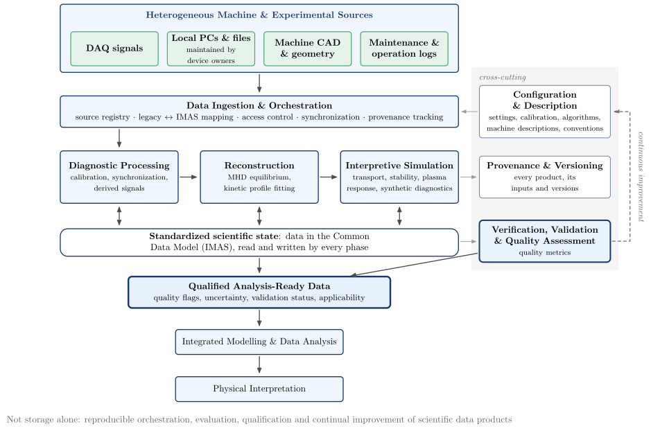
vaft.diagram.scientific_workflow()A managed scientific processing pipeline: heterogeneous sources to qualified, analysis-ready data.
vaft.diagram.scientific_workflow(*, labels=True)Formats .svg .tex .pdf the SVG above is committed; build the others locally
import vaft.diagram
d = vaft.diagram.scientific_workflow()
d.tikz # the TikZ document as text
d.save("scientific_workflow.svg") # rendered vector image, the canonical artifact; needs latex, dvisvgm
d.save("scientific_workflow.tex") # the complete TikZ document, the text source
d.save("scientific_workflow.pdf") # vector PDF; needs pdflatexinteroperability_layers
1 asset
source
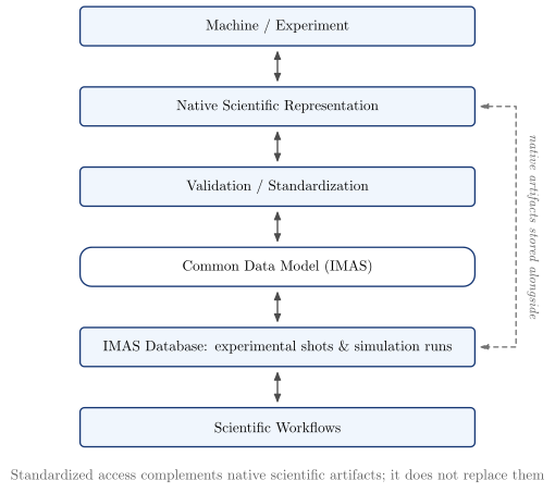
vaft.diagram.interoperability_layers()Interoperability as layers: from the machine to scientific workflows, in both directions.
vaft.diagram.interoperability_layers(*, labels=True)Show source vaft/diagram/_vaft_concepts.py, lines 355–389
def interoperability_layers(*, labels: bool = True) -> Diagram:
r"""Interoperability as layers: from the machine to scientific workflows, in both directions.
Machine, native scientific representation, validation and
standardization, the Common Data Model (IMAS), the IMAS database and scientific
workflows, each exchanging with its neighbours. Native artifacts are
kept beside the standardized representation -- the dashed path -- so
standardization complements the native form rather than replacing it.
"""
labels = _check_labels(labels)
items: List = []
edges: List = []
w, h, step = 9.6, 0.95, 1.95
boxes: Dict[str, Box] = {}
for i, (key, text) in enumerate(LAYERS):
style = "concept state" if key == "imas" else "concept box"
b = box(0.0, -i * step, w, h, text, style=style, role=f"layer:{key}")
boxes[key] = b
items += list(b.items)
keys = [k for k, _ in LAYERS]
for a, b in zip(keys, keys[1:]):
_edge(items, edges, boxes[a], boxes[b], a, b, both=True)
# native artifacts stay available next to the standard: a path around the standardization
native, db = boxes["native"], boxes["database"]
x = 0.5 * w + 1.0
items.append(Polyline.of([(0.5 * w + 0.08, native.y), (x, native.y), (x, db.y), (0.5 * w + 0.08, db.y)],
"connector feedback,<->", role="edge:native->database"))
_record(edges, "native", "database", "complement")
if labels:
items.append(Label((x + 0.15, 0.5 * (native.y + db.y)), "native artifacts stored alongside",
"concept annotation,rotate=-90", anchor="south", role="complement"))
items.append(Label((0.0, -(len(LAYERS) - 1) * step - 0.9), "Standardized access complements native "
"scientific artifacts; it does not replace them", "note", anchor="north", role="note"))
return Diagram("interoperability_layers", Scene(tuple(items)),
model={"layers": tuple(keys), "edges": tuple(edges)})Formats .svg .tex .pdf the SVG above is committed; build the others locally
import vaft.diagram
d = vaft.diagram.interoperability_layers()
d.tikz # the TikZ document as text
d.save("interoperability_layers.svg") # rendered vector image, the canonical artifact; needs latex, dvisvgm
d.save("interoperability_layers.tex") # the complete TikZ document, the text source
d.save("interoperability_layers.pdf") # vector PDF; needs pdflatexscientific_provenance_chain
1 asset
source
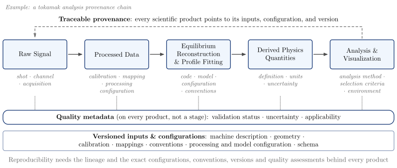
vaft.diagram.scientific_provenance_chain()Traceable provenance: every scientific product points to its inputs, configuration and version.
vaft.diagram.scientific_provenance_chain(*, labels=True)Show source vaft/diagram/_vaft_concepts.py, lines 410–465
def scientific_provenance_chain(*, labels: bool = True) -> Diagram:
r"""Traceable provenance: every scientific product points to its inputs, configuration and version.
Raw signal, processed data, equilibrium reconstruction and profile
fitting, derived physics quantities, analysis and visualization. Each
step records what produced it; calibration, mapping and processing
configuration are provenance of the raw-to-processed step, not a stage
of their own. Two kinds of metadata are kept apart: versioned
provenance (machine description, geometry, calibration, mappings,
conventions, configurations, schema) and quality metadata (validation
status, uncertainty, applicability), which cuts across every product
rather than being a final stage. Reproducibility needs both the lineage
and the exact configurations, conventions, versions and quality
assessments behind each quantity.
"""
labels = _check_labels(labels)
items: List = []
edges: List = []
w, h, gap = 3.4, 1.55, 0.95
boxes: List[Box] = []
for i, (key, text, records) in enumerate(PROVENANCE):
b = box(i * (w + gap), 0.0, w, h, text, role=f"step:{key}")
boxes.append(b)
items += list(b.items)
items.append(Label((b.x, -0.5 * h - 0.15), _dotted(records.split(", ")),
"concept annotation,text width=3.2cm", anchor="north", role=f"record:{key}"))
for (k0, _, _), (k1, _, _), a, b in zip(PROVENANCE, PROVENANCE[1:], boxes, boxes[1:]):
_edge(items, edges, a, b, k0, k1)
first, last = boxes[0], boxes[-1]
left, right = first.x - 0.5 * w, last.x + 0.5 * w
y = 0.5 * h + 0.7
items.append(Polyline.of([(last.x, 0.5 * h + 0.08), (last.x, y), (first.x, y), (first.x, 0.5 * h + 0.08)],
"connector feedback", role="trace"))
items.append(Label((left, y + 0.75), "Example: a tokamak analysis provenance chain", "concept band label",
anchor="south west", role="example"))
items.append(Label((0.5 * (left + right), y + 0.1), "\\textbf{Traceable provenance}: every scientific product "
"points to its inputs, configuration, and version", "concept plain", anchor="south",
role="trace"))
# quality metadata cuts across every product
qy = -3.35
quality = box(0.5 * (left + right), qy, right - left, 0.75, "\\textbf{Quality metadata} (on every product, not "
"a stage): " + _dotted(QUALITY), style="concept state", role="quality", latex=True)
items += list(quality.items)
for b in boxes:
items.append(Polyline.of([(b.x, -0.5 * h - 1.45), (b.x, qy + 0.375)], "concept tick", role="quality"))
versioned = box(0.5 * (left + right), qy - 1.25, right - left, 1.05, "\\textbf{Versioned inputs \\& configurations}: "
+ _dotted(VERSIONED), style="concept leaf", role="versioned", latex=True)
items += list(versioned.items)
if labels:
items.append(Label((0.5 * (left + right), qy - 2.0), "Reproducibility needs the lineage and the exact "
"configurations, conventions, versions and quality assessments behind every product",
"note", anchor="north", role="note"))
return Diagram("scientific_provenance_chain", Scene(tuple(items)),
model={"steps": tuple(k for k, _, _ in PROVENANCE), "edges": tuple(edges),
"records": {k: r for k, _, r in PROVENANCE}, "trace": ("analysis", "raw"),
"versioned": VERSIONED, "quality": QUALITY})Formats .svg .tex .pdf the SVG above is committed; build the others locally
import vaft.diagram
d = vaft.diagram.scientific_provenance_chain()
d.tikz # the TikZ document as text
d.save("scientific_provenance_chain.svg") # rendered vector image, the canonical artifact; needs latex, dvisvgm
d.save("scientific_provenance_chain.tex") # the complete TikZ document, the text source
d.save("scientific_provenance_chain.pdf") # vector PDF; needs pdflatexplasma_state_provenance
1 asset
source
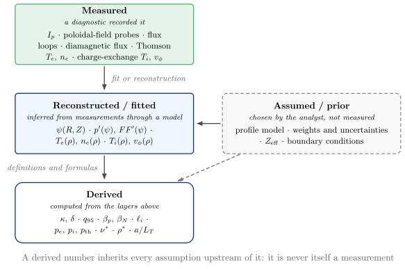
vaft.diagram.plasma_state_provenance()Where each quantity of a plasma state comes from: measured, reconstructed, assumed or derived.
vaft.diagram.plasma_state_provenance(*, labels=True)Show source vaft/diagram/_vaft_concepts.py, lines 489–529
def plasma_state_provenance(*, labels: bool = True) -> Diagram:
r"""Where each quantity of a plasma state comes from: measured, reconstructed, assumed or derived.
Measurements (plasma current, magnetic probes and loops, diamagnetic
flux, Thomson and charge-exchange profiles) enter a reconstruction or a
profile fit, which also takes assumptions the data cannot supply: the
profile model, the weights and uncertainties, the effective charge and
the boundary conditions; some assumptions (an effective charge in a
collisionality, $n_i = n_e$ in an ion pressure) enter only the derivation
itself. The fitted fields and profiles feed the derived
descriptors (shape, $q_{95}$, $\beta$, $\ell_i$, pressures, collisionality,
normalized gyroradius and gradient lengths). A derived number inherits
every assumption made upstream of it, so it is never itself a measurement.
"""
labels = _check_labels(labels)
items: List = []
edges: List = []
w, h, step, side = 6.8, 2.3, 3.4, 7.9
positions = {"measured": (0.0, 0.0), "reconstructed": (0.0, -step), "assumed": (side, -step),
"derived": (0.0, -2 * step)}
boxes: Dict[str, Box] = {}
for key, title, meaning, examples, style in STATE_LAYERS:
x, y = positions[key]
b = box(x, y, w, h, _layer_text(title, meaning, examples), style=style, role=f"layer:{key}", latex=True)
boxes[key] = b
items += list(b.items)
_down_or_up(items, edges, boxes["measured"], boxes["reconstructed"], "measured", "reconstructed")
_edge(items, edges, boxes["assumed"], boxes["reconstructed"], "assumed", "reconstructed")
_down_or_up(items, edges, boxes["reconstructed"], boxes["derived"], "reconstructed", "derived")
# some assumptions enter only the derivation: a chosen Z_eff in a collisionality, n_i = n_e in p_i
_edge(items, edges, boxes["assumed"], boxes["derived"], "assumed", "derived", style="connector feedback")
if labels:
items.append(Label((0.15, -0.5 * step), "fit or reconstruction", "concept annotation", anchor="west",
role="note"))
items.append(Label((-0.15, -1.5 * step), "definitions and formulas", "concept annotation", anchor="east",
role="note"))
items.append(Label((0.5 * side, -2 * step - 0.5 * h - 0.3), "A derived number inherits every assumption "
"upstream of it: it is never itself a measurement", "note", anchor="north", role="note"))
return Diagram("plasma_state_provenance", Scene(tuple(items)),
model={"layers": tuple(k for k, *_ in STATE_LAYERS), "edges": tuple(edges),
"examples": {k: e for k, _, _, e, _ in STATE_LAYERS}})Formats .svg .tex .pdf the SVG above is committed; build the others locally
import vaft.diagram
d = vaft.diagram.plasma_state_provenance()
d.tikz # the TikZ document as text
d.save("plasma_state_provenance.svg") # rendered vector image, the canonical artifact; needs latex, dvisvgm
d.save("plasma_state_provenance.tex") # the complete TikZ document, the text source
d.save("plasma_state_provenance.pdf") # vector PDF; needs pdflatexscientific_infrastructure_principles
1 asset
source
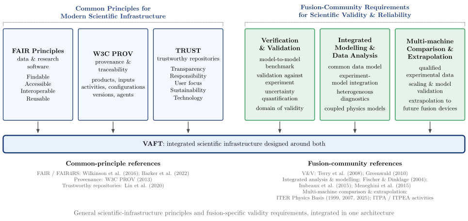
vaft.diagram.scientific_infrastructure_principles()Two complementary foundations of VAFT, converging on one infrastructure.
vaft.diagram.scientific_infrastructure_principles(*, labels=True)Show source vaft/diagram/_vaft_concepts.py, lines 564–629
def scientific_infrastructure_principles(*, labels: bool = True) -> Diagram:
r"""Two complementary foundations of VAFT, converging on one infrastructure.
On the left, common principles for modern scientific infrastructure,
adopted from established cross-disciplinary practice: FAIR for data and
research software, W3C PROV for provenance and traceability, TRUST for
trustworthy repository operation. On the right, the methodological
requirements and practice established in the fusion community, in three
blocks that balance the left without a one-to-one correspondence:
verification and validation (model-to-model benchmarks, validation
against experiment, uncertainty quantification, domain of validity);
integrated modelling and data analysis, starting from a common data
model; multi-machine comparison and extrapolation. The two headings are
parallel, and each block converges independently on VAFT, an
architecture designed around both (not a claim of complete compliance).
Beneath each side, its references grouped by block; FAIR4RS is named
there, next to FAIR.
"""
labels = _check_labels(labels)
items: List = []
edges: List = []
w, gap, h, split = 3.8, 0.3, 5.0, 1.2
side = 3 * w + 2 * gap
total = 2 * side + split
x0 = -0.5 * total
left_c, right_c = x0 + 0.5 * side, 0.5 * total - 0.5 * side
vaft = box(0.0, -0.5 * h - 1.3, total, 0.95, "\\textbf{VAFT}: integrated scientific infrastructure designed around both",
style="concept strong", role="node:vaft", latex=True)
items += list(vaft.items)
blocks = [(key, _titled(title, sub) + "\\\\[5pt]{\\small " + "\\\\".join(map(escape_latex, content)) + "}",
"concept pillar", "principle") for key, title, sub, content in COMMON_PRINCIPLES]
for key, title, content in FUSION_REQUIREMENTS:
lines = list(map(escape_latex, content))
blocks.append((key, _titled(title) + "\\\\[6pt]{\\small " + "\\\\[3pt]".join(lines) + "}",
"concept requirement", "requirement"))
for i, (key, body, style, kind) in enumerate(blocks):
x = x0 + 0.5 * w + i * (w + gap) + (split - gap if i >= 3 else 0.0)
b = box(x, 0.0, w, h, body, style=style, role=f"{kind}:{key}", latex=True)
items += list(b.items)
_down_or_up(items, edges, b, vaft, f"{kind}:{key}", "vaft")
# parallel headings over the two sides
top = 0.5 * h + 0.15
for c, text, role in ((left_c, "Common Principles for\\\\Modern Scientific Infrastructure", "heading:common"),
(right_c, "Fusion-Community Requirements\\\\for Scientific Validity \\& Reliability",
"heading:fusion")):
lo, hi = c - 0.5 * side, c + 0.5 * side
items += [Polyline.of([(lo, top), (lo, top + 0.2), (hi, top + 0.2), (hi, top)], "concept tick", role=role),
Label((c, top + 0.3), text, "concept group title,align=center", anchor="south", role=role)]
# compact foundations and references beneath each side
fy = vaft.y - 0.8
items += [Label((left_c, fy), "\\textbf{Common-principle references}", "concept plain", anchor="north",
role="footer:common"),
Label((left_c, fy - 0.55), "\\\\".join(map(escape_latex, PRINCIPLE_REFERENCES)), "concept reference",
anchor="north", role="references"),
Label((right_c, fy), "\\textbf{Fusion-community references}", "concept plain", anchor="north",
role="footer:fusion"),
Label((right_c, fy - 0.55), "\\\\".join(map(escape_latex, FUSION_REFERENCES)), "concept reference",
anchor="north", role="fusion_references")]
if labels:
items.append(Label((0.0, fy - 2.7), "General scientific-infrastructure principles and fusion-specific validity "
"requirements, integrated in one architecture", "note", anchor="north", role="note"))
return Diagram("scientific_infrastructure_principles", Scene(tuple(items)),
model={"principles": tuple(k for k, *_ in COMMON_PRINCIPLES),
"requirements": tuple(k for k, *_ in FUSION_REQUIREMENTS),
"references": PRINCIPLE_REFERENCES, "fusion_references": FUSION_REFERENCES,
"edges": tuple(edges)})Formats .svg .tex .pdf the SVG above is committed; build the others locally
import vaft.diagram
d = vaft.diagram.scientific_infrastructure_principles()
d.tikz # the TikZ document as text
d.save("scientific_infrastructure_principles.svg") # rendered vector image, the canonical artifact; needs latex, dvisvgm
d.save("scientific_infrastructure_principles.tex") # the complete TikZ document, the text source
d.save("scientific_infrastructure_principles.pdf") # vector PDF; needs pdflatexmachine_agnostic_architecture
1 asset
source
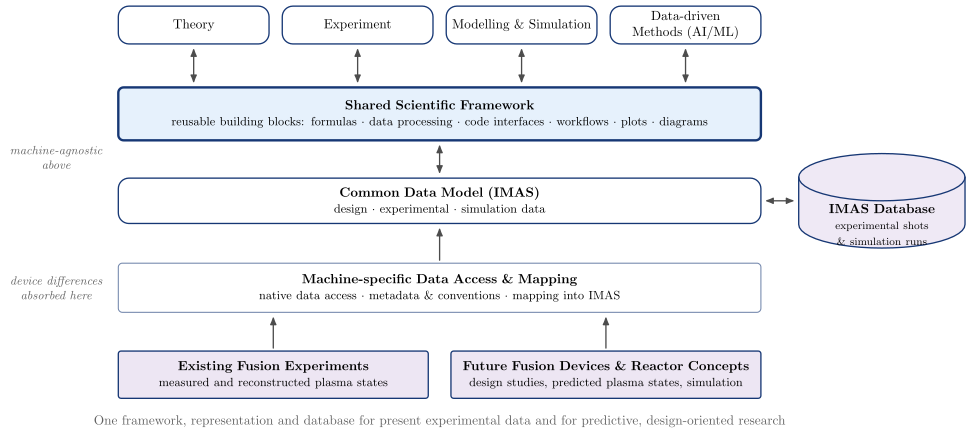
vaft.diagram.machine_agnostic_architecture()A machine-agnostic scientific framework for integrated fusion research.
vaft.diagram.machine_agnostic_architecture(*, labels=True)Show source vaft/diagram/_vaft_concepts.py, lines 643–705
def machine_agnostic_architecture(*, labels: bool = True) -> Diagram:
r"""A machine-agnostic scientific framework for integrated fusion research.
Theory, experiment, modelling and simulation, and data-driven methods
share one scientific framework of reusable building blocks -- formulas,
data processing, code interfaces, workflows, plots, diagrams. Below it,
one Common Data Model (IMAS) describes design, experimental and
simulation data alike, and is stored and reused in the IMAS database of
experimental shots and simulation runs. Machine-specific data access and
mapping (native access, metadata and conventions, mapping into IMAS)
absorbs the differences between devices, so that everything above stays
machine-agnostic. The same architecture serves two domains: existing
fusion experiments (measured and reconstructed plasma states) and future
fusion devices and reactor concepts (design studies, predicted states,
simulation). No device is named.
"""
labels = _check_labels(labels)
items: List = []
edges: List = []
span = 17.0
gap = 0.35
rw = (span - 3 * gap) / 4
research: Dict[str, Box] = {}
for i, (key, text) in enumerate(RESEARCH):
x = -0.5 * span + 0.5 * rw + i * (rw + gap)
research[key] = box(x, 8.65, rw, 1.0, text, style="concept state", role=f"research:{key}")
items += list(research[key].items)
framework = box(0.0, 6.3, span, 1.4, "\\textbf{Shared Scientific Framework}\\\\{\\small reusable building "
"blocks: formulas $\\cdot$ data processing $\\cdot$ code interfaces $\\cdot$ workflows $\\cdot$ "
"plots $\\cdot$ diagrams}", style="concept strong", role="layer:framework", latex=True)
standard = box(0.0, 4.0, span, 1.2, "\\textbf{Common Data Model (IMAS)}\\\\{\\small design "
"$\\cdot$ experimental $\\cdot$ simulation data}", style="concept state", role="layer:standard",
latex=True)
mapping = box(0.0, 1.7, span, 1.3, "\\textbf{Machine-specific Data Access \\& Mapping}\\\\{\\small native "
"data access $\\cdot$ metadata \\& conventions $\\cdot$ mapping into IMAS}", style="concept leaf",
role="layer:mapping", latex=True)
items += list(framework.items) + list(standard.items) + list(mapping.items)
for key, r in research.items():
items.append(Arrow((r.x, framework.y + 0.7 + 0.08), (r.x, r.y - 0.5 - 0.08), "connector both",
role=f"edge:framework->research:{key}", both=True))
_record(edges, "framework", f"research:{key}", "both")
_edge(items, edges, standard, framework, "standard", "framework", both=True)
_edge(items, edges, mapping, standard, "mapping", "standard")
db = database(0.5 * span + 3.2, 4.0, 4.4, 2.5, DATABASE_TEXT, role="node:database", latex=True)
items += list(db.items)
_edge(items, edges, standard, db, "standard", "database", both=True)
dw = 0.5 * (span - 0.6)
for (key, title, sub), x in zip(DOMAINS, (-0.25 * span - 0.15, 0.25 * span + 0.15)):
d = box(x, -0.6, dw, 1.25, _titled(title, sub), style="concept base", role=f"domain:{key}", latex=True)
items += list(d.items)
items.append(Arrow((x, d.y + 0.625 + 0.08), (x, mapping.y - 0.65 - 0.08), "connector",
role=f"edge:domain:{key}->mapping"))
_record(edges, f"domain:{key}", "mapping", "forward")
items.append(Label((-0.5 * span - 0.3, mapping.y), "device differences\\\\absorbed here", "concept annotation",
anchor="east", role="absorb"))
items.append(Label((-0.5 * span - 0.3, 0.5 * (framework.y + standard.y)), "machine-agnostic\\\\above",
"concept annotation", anchor="east", role="absorb"))
if labels:
items.append(Label((0.0, -1.55), "One framework, representation and database for present experimental data "
"and for predictive, design-oriented research", "note", anchor="north", role="note"))
return Diagram("machine_agnostic_architecture", Scene(tuple(items)),
model={"research": tuple(k for k, _ in RESEARCH), "domains": tuple(k for k, _, _ in DOMAINS),
"edges": tuple(edges)})Formats .svg .tex .pdf the SVG above is committed; build the others locally
import vaft.diagram
d = vaft.diagram.machine_agnostic_architecture()
d.tikz # the TikZ document as text
d.save("machine_agnostic_architecture.svg") # rendered vector image, the canonical artifact; needs latex, dvisvgm
d.save("machine_agnostic_architecture.tex") # the complete TikZ document, the text source
d.save("machine_agnostic_architecture.pdf") # vector PDF; needs pdflatexexperiment_modeling_theory_data_network
3 assets
source
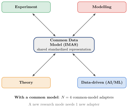
vaft.diagram.experiment_modeling_theory_data_network()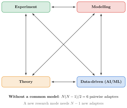
vaft.diagram.experiment_modeling_theory_data_network(communication='point_to_point')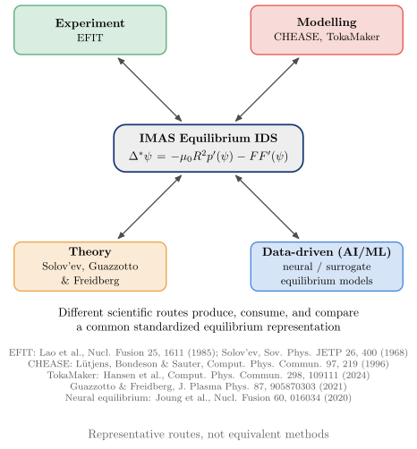
vaft.diagram.experiment_modeling_theory_data_network(communication='equilibrium')Why a common fusion data model: four research modes, pairwise against a shared representation.
vaft.diagram.experiment_modeling_theory_data_network(communication='common_model', *, labels=True)Show source vaft/diagram/_vaft_concepts.py, lines 761–817
def experiment_modeling_theory_data_network(communication: str = "common_model", *,
labels: bool = True) -> Diagram:
r"""Why a common fusion data model: four research modes, pairwise against a shared representation.
``communication`` selects one diagram of a three-step sequence:
``"point_to_point"``
experiment, modelling, theory and data-driven (AI/ML) research
connected pairwise -- without a common model, $N(N-1)/2$ pairwise
adapters, and a new mode needs $N-1$ more;
``"common_model"``
the same four modes each reading from and writing to one Common Data
Model (IMAS) -- $N$ common-model adapters, and a new mode needs one;
``"equilibrium"``
the concrete tokamak case: the IMAS equilibrium IDS at the centre and
representative routes of each mode (EFIT; CHEASE, TokaMaker;
Solov'ev, Guazzotto & Freidberg; neural / surrogate equilibrium
models). The routes produce, consume and compare a common
standardized equilibrium representation; they are not equivalent
methods. Compact references sit beneath.
"""
labels = _check_labels(labels)
if communication not in _COMMUNICATION:
raise ValueError(f"communication must be one of {_COMMUNICATION}, not {communication!r}")
items: List = []
edges: List = []
d = _MODE_OFFSET
example = communication == "equilibrium"
nodes = _research_modes(items, example)
keys = [k for k, _, _ in ACTIVITIES]
n = len(keys)
if communication == "point_to_point":
for i, a in enumerate(keys):
for b in keys[i + 1:]:
_edge(items, edges, nodes[a], nodes[b], a, b, both=True)
adapters = n * (n - 1) // 2
caption = f"\\textbf{{Without a common model}}: $N(N-1)/2 = {adapters}$ pairwise adapters"
note = "A new research mode needs $N-1$ new adapters"
else:
_common_hub(items, edges, nodes, example)
adapters = n
caption = (f"\\textbf{{With a common model}}: $N = {adapters}$ common-model adapters" if not example else
"Different scientific routes produce, consume, and compare\\\\a common standardized equilibrium "
"representation")
note = ("A new research mode needs 1 new adapter" if not example else
"Representative routes, not equivalent methods")
items.append(Label((0.0, -d - 1.1), caption, "concept plain", anchor="north", role="caption"))
if example:
lines = ("; ".join(EQUILIBRIUM_REFERENCES[i] for i in group) for group in _REFERENCE_LINES)
items.append(Label((0.0, -d - 2.3), "\\\\".join(lines), "concept reference", anchor="north",
role="references"))
if labels:
items.append(Label((0.0, -d - (4.7 if example else 1.75)), note, "note", anchor="north", role="note"))
return Diagram("experiment_modeling_theory_data_network", Scene(tuple(items)),
model={"communication": communication, "nodes": tuple(keys), "edges": tuple(edges),
"adapters": adapters,
"routes": dict(EQUILIBRIUM_ROUTES) if example else {}})Formats .svg .tex .pdf the SVG above is committed; build the others locally
import vaft.diagram
d = vaft.diagram.experiment_modeling_theory_data_network()
d.tikz # the TikZ document as text
d.save("experiment_modeling_theory_data_network.svg") # rendered vector image, the canonical artifact; needs latex, dvisvgm
d.save("experiment_modeling_theory_data_network.tex") # the complete TikZ document, the text source
d.save("experiment_modeling_theory_data_network.pdf") # vector PDF; needs pdflatexintegrated_scientific_framework
2 assets
source
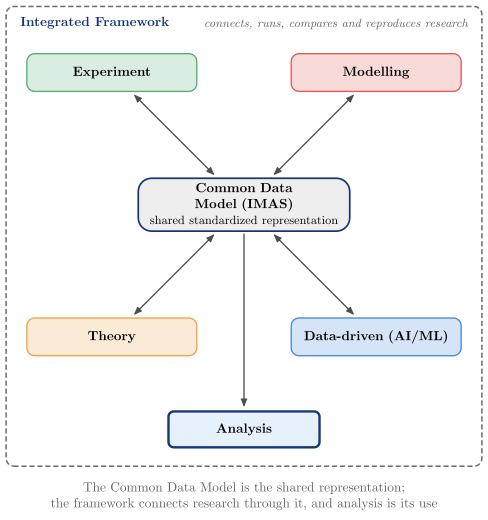
vaft.diagram.integrated_scientific_framework()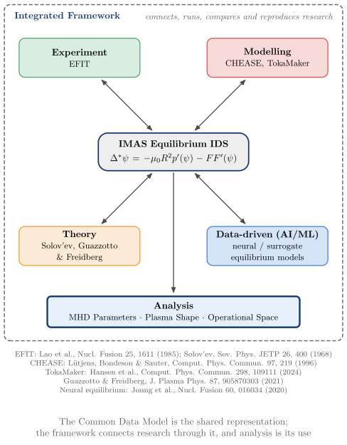
vaft.diagram.integrated_scientific_framework(domain='equilibrium')The research modes and their common state inside one integrated framework, serving analysis (#1698).
vaft.diagram.integrated_scientific_framework(domain=None, *, labels=True)Show source vaft/diagram/_vaft_concepts.py, lines 828–886
def integrated_scientific_framework(domain: Optional[str] = None, *, labels: bool = True) -> Diagram:
r"""The research modes and their common state inside one integrated framework, serving analysis (#1698).
The four research modes and the Common Data Model (IMAS) sit exactly as in
``experiment_modeling_theory_data_network("common_model")``, inside an
Integrated Framework boundary, and the shared state feeds one downstream
Analysis node. Three concepts are kept apart: the Common Data Model is the
shared representation; the framework connects, runs, compares and
reproduces research through it; analysis is the scientific use of the
integrated state.
``domain="equilibrium"`` specialises the figure: the representative
equilibrium routes of each mode and the IMAS equilibrium IDS, with an
analysis of MHD parameters, plasma shape and operational space -- the
equilibrium-derived descriptors. Stability codes are downstream models of
the equilibrium and stay out of it. Compact references sit beneath.
"""
labels = _check_labels(labels)
if domain not in _FRAMEWORK_DOMAINS:
raise ValueError(f"domain must be one of {_FRAMEWORK_DOMAINS}, not {domain!r}")
example = domain == "equilibrium"
d = _MODE_OFFSET
items: List = []
edges: List = []
# the framework boundary first, so everything else is drawn over it
frame_x, frame_top = d + 2.25 + 0.55, d + (0.725 if example else 0.5) + 1.25
analysis_y = -d - 2.45
analysis_h = 1.15 if example else 0.95
frame_bottom = analysis_y - 0.5 * analysis_h - 0.5
items.append(Polyline.of([(-frame_x, frame_bottom), (frame_x, frame_bottom), (frame_x, frame_top),
(-frame_x, frame_top)], "concept frame", role="framework", closed=True))
items.append(Label((-frame_x + 0.25, frame_top - 0.15), "\\textbf{Integrated Framework}", "concept group title",
anchor="north west", role="framework"))
items.append(Label((frame_x - 0.25, frame_top - 0.2), "connects, runs, compares and reproduces research",
"concept annotation", anchor="north east", role="framework"))
nodes = _research_modes(items, example)
hub = _common_hub(items, edges, nodes, example)
body = "\\textbf{Analysis}"
if example:
body += "\\\\{\\small " + " $\\cdot$ ".join(escape_latex(t) for _, t in EQUILIBRIUM_ANALYSIS) + "}"
analysis = box(0.0, analysis_y, 9.4 if example else 4.0, analysis_h, body, style="concept strong",
role="node:analysis", latex=True)
items += list(analysis.items)
_down_or_up(items, edges, hub, analysis, "hub", "analysis")
if example:
lines = ("; ".join(EQUILIBRIUM_REFERENCES[i] for i in group) for group in _REFERENCE_LINES)
items.append(Label((0.0, frame_bottom - 0.25), "\\\\".join(lines), "concept reference", anchor="north",
role="references"))
if labels:
note = ("The Common Data Model is the shared representation;\\\\the framework connects research through it, "
"and analysis is its use")
items.append(Label((0.0, frame_bottom - (2.75 if example else 0.3)), note, "note", anchor="north", role="note"))
return Diagram("integrated_scientific_framework", Scene(tuple(items)),
model={"framework": "integrated", "domain": domain,
"activities": tuple(k for k, _, _ in ACTIVITIES),
"shared_state": "equilibrium" if example else "common_data_model",
"analysis": "analysis",
"analysis_categories": tuple(k for k, _ in EQUILIBRIUM_ANALYSIS) if example else (),
"routes": dict(EQUILIBRIUM_ROUTES) if example else {}, "edges": tuple(edges)})Formats .svg .tex .pdf the SVG above is committed; build the others locally
import vaft.diagram
d = vaft.diagram.integrated_scientific_framework()
d.tikz # the TikZ document as text
d.save("integrated_scientific_framework.svg") # rendered vector image, the canonical artifact; needs latex, dvisvgm
d.save("integrated_scientific_framework.tex") # the complete TikZ document, the text source
d.save("integrated_scientific_framework.pdf") # vector PDF; needs pdflatexhuman_ai_interface
1 asset
source
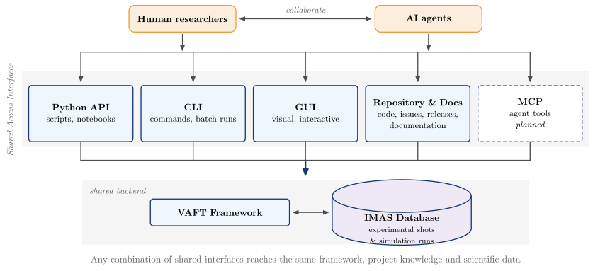
vaft.diagram.human_ai_interface()Human-AI collaborative access: who, how, and what.
vaft.diagram.human_ai_interface(*, labels=True)Show source vaft/diagram/_vaft_concepts.py, lines 899–959
def human_ai_interface(*, labels: bool = True) -> Diagram:
r"""Human-AI collaborative access: who, how, and what.
Human researchers and AI agents collaborate (a two-way relationship,
not two isolated user classes) and reach one shared interface layer:
the Python API (scripts, notebooks), the CLI (commands, batch runs), a
GUI (visual, interactive), the repository and docs (code, issues,
releases and documentation) and MCP (agent tools; planned).
Every interface reaches the same backend -- the VAFT framework and its
scientific data repository -- and none is reserved for one kind of user.
"""
labels = _check_labels(labels)
items: List = []
edges: List = []
w, gap = 3.9, 0.3
span = len(INTERFACES) * w + (len(INTERFACES) - 1) * gap
human = box(-4.6, 5.0, 4.0, 1.0, "\\textbf{Human researchers}", style="concept actor", role="actor:human",
latex=True)
agent = box(4.6, 5.0, 4.0, 1.0, "\\textbf{AI agents}", style="concept actor", role="actor:agent", latex=True)
items += list(human.items) + list(agent.items)
_edge(items, edges, human, agent, "actor:human", "actor:agent", both=True)
items.append(Label((0.0, 5.1), "collaborate", "concept annotation", anchor="south", role="collaborate"))
bar_y = 3.75
xs = [-0.5 * span + 0.5 * w + i * (w + gap) for i in range(len(INTERFACES))]
items.append(Polyline.of([(xs[0], bar_y), (xs[-1], bar_y)], "connector line", role="access"))
for key, actor in (("human", human), ("agent", agent)):
items.append(Arrow((actor.x, actor.y - 0.5 - 0.08), (actor.x, bar_y), "connector",
role=f"edge:actor:{key}->access"))
_record(edges, f"actor:{key}", "access", "forward")
# the shared interface layer, labelled, collected into one connection to the backend
items += band(-0.5 * span - 0.25, 0.5 * span + 0.25, 0.2, 3.05, role="layer:interfaces")
items.append(Label((-0.5 * span - 0.4, 1.6), "Shared Access Interfaces", "concept band label,rotate=90", anchor="south",
role="layer:interfaces"))
collector_y, backend_top, backend_bottom = -0.3, -1.05, -3.45
items.append(Polyline.of([(xs[0], collector_y), (xs[-1], collector_y)], "connector line", role="collector"))
items.append(Arrow((0.0, collector_y), (0.0, backend_top + 0.08), "connector strong",
role="edge:interfaces->backend"))
_record(edges, "interfaces", "backend", "forward")
items += band(-0.5 * span + 2.0, 0.5 * span - 2.0, backend_bottom, backend_top, "shared backend", role="backend")
framework = box(-3.2, -2.25, 5.2, 1.0, "\\textbf{VAFT Framework}", role="node:framework", latex=True)
repository = database(3.6, -2.25, 5.2, 2.45, DATABASE_TEXT, role="node:repository", latex=True)
items += list(framework.items) + list(repository.items)
_edge(items, edges, framework, repository, "framework", "repository", both=True)
for (key, name, use, planned), x in zip(INTERFACES, xs):
body = _titled(name, use)
if planned:
body += "\\\\{\\small\\itshape planned}"
b = box(x, 1.45, w, 2.1, body, style="concept group" if planned else "concept box",
role=f"interface:{key}", latex=True)
items += list(b.items)
items.append(Arrow((x, bar_y), (x, b.y + 1.05 + 0.08), "connector", role=f"edge:access->interface:{key}"))
_record(edges, "access", f"interface:{key}", "forward")
items.append(Polyline.of([(x, b.y - 1.05), (x, collector_y)], "connector line", role=f"edge:interface:{key}->interfaces"))
_record(edges, f"interface:{key}", "interfaces", "forward")
if labels:
items.append(Label((0.0, backend_bottom - 0.3), "Any combination of shared interfaces reaches the same "
"framework, project knowledge and scientific data", "note", anchor="north", role="note"))
return Diagram("human_ai_interface", Scene(tuple(items)),
model={"actors": ("human", "agent"), "interfaces": tuple(k for k, *_ in INTERFACES),
"planned": tuple(k for k, *_, p in INTERFACES if p), "backend": ("framework", "repository"),
"edges": tuple(edges)})Formats .svg .tex .pdf the SVG above is committed; build the others locally
import vaft.diagram
d = vaft.diagram.human_ai_interface()
d.tikz # the TikZ document as text
d.save("human_ai_interface.svg") # rendered vector image, the canonical artifact; needs latex, dvisvgm
d.save("human_ai_interface.tex") # the complete TikZ document, the text source
d.save("human_ai_interface.pdf") # vector PDF; needs pdflatexmachine_research_archive
1 asset
source
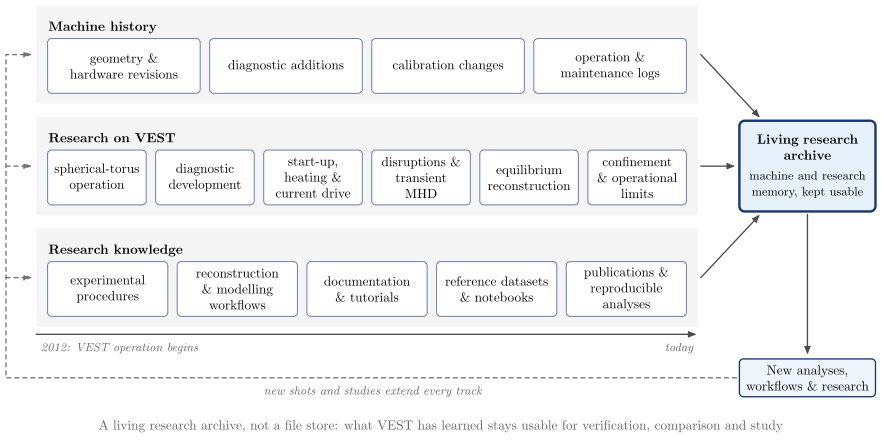
vaft.diagram.machine_research_archive()The machine and research archive: VEST’s institutional and scientific memory since 2012.
vaft.diagram.machine_research_archive(*, labels=True)Show source vaft/diagram/_vaft_concepts.py, lines 975–1046
def machine_research_archive(*, labels: bool = True) -> Diagram:
r"""The machine and research archive: VEST's institutional and scientific memory since 2012.
Three tracks run from the start of VEST operation in 2012 to today:
machine history (geometry and hardware revisions, diagnostic additions,
calibration changes, operation and maintenance logs); the research
actually carried out on VEST, after the README's "Research historically
performed on VEST" (spherical-torus operation, diagnostic development,
start-up, heating and current drive, disruptions and transient MHD,
equilibrium reconstruction, confinement and operational limits); and
research knowledge (procedures, reconstruction and modelling workflows,
documentation and tutorials, reference datasets and notebooks,
publications and reproducible analyses). All three feed one living
research archive, which is not the end of the pipeline: new analyses,
workflows and research build on it and extend every track. No dates are
drawn beyond the start of operation; the figure shows what accumulates,
not when.
"""
labels = _check_labels(labels)
items: List = []
edges: List = []
x0, x1 = 0.0, 17.5
track_y = {"machine": 6.55, "studies": 3.6, "research": 0.65}
for key, title, entries in ARCHIVE_TRACKS:
y = track_y[key]
items += band(x0, x1, y - 1.3, y + 1.3, role=f"track:{key}")
items.append(Label((x0 + 0.2, y + 1.0), "\\textbf{" + escape_latex(title) + "}", "concept plain",
anchor="north west", role=f"track:{key}"))
n = len(entries)
w = (x1 - x0 - 0.6 - (n - 1) * 0.25) / n
for i, text in enumerate(entries):
b = box(x0 + 0.3 + 0.5 * w + i * (w + 0.25), y - 0.3, w, 1.45, text, style="concept leaf",
role=f"entry:{key}:{i}")
items += list(b.items)
archive = box(x1 + 2.9, track_y["studies"], 3.6, 2.4,
"\\textbf{Living research archive}\\\\[3pt]{\\small machine and research memory, kept usable}",
style="concept strong", role="node:archive", latex=True)
items += list(archive.items)
for key, y in track_y.items(): # every track ends in the one archive
bx, by = archive.boundary_point((x1, y))
sx, sy = x1 + 0.08, y
length = math.hypot(bx - sx, by - sy)
end = (float(bx - 0.08 * (bx - sx) / length), float(by - 0.08 * (by - sy) / length))
items.append(Arrow((sx, sy), end, "connector", role=f"edge:track:{key}->archive"))
_record(edges, f"track:{key}", "archive", "forward")
research = box(archive.x, -2.0, 3.6, 1.0, "New analyses, workflows & research", role="node:next")
items += list(research.items)
_down_or_up(items, edges, archive, research, "archive", "next")
# the archive is an input: new work extends every track
y_back = -2.0
xl = x0 - 0.8
items.append(Polyline.of([(research.x - 0.5 * research.width - 0.08, y_back), (xl, y_back), (xl, track_y["machine"]),
(x0 - 0.08, track_y["machine"])], "connector feedback", role="edge:next->track:machine"))
_record(edges, "next", "track:machine", "feedback")
for key in ("studies", "research"):
items.append(Arrow((xl, track_y[key]), (x0 - 0.08, track_y[key]), "connector feedback",
role=f"edge:next->track:{key}"))
_record(edges, "next", f"track:{key}", "feedback")
items.append(Label((0.5 * (xl + research.x - 0.5 * research.width), y_back - 0.1),
"new shots and studies extend every track", "concept annotation", anchor="north",
role="feedback_label"))
items += [Arrow((x0, -0.85), (x1, -0.85), "connector line,->", role="time"),
Label((x0, -0.95), "2012: VEST operation begins", "concept annotation", anchor="north west",
role="time"),
Label((x1, -0.95), "today", "concept annotation", anchor="north east", role="time")]
if labels:
items.append(Label((0.5 * (xl + archive.x + 1.8), -3.0), "A living research archive, not a file store: "
"what VEST has learned stays usable for verification, comparison and study",
"note", anchor="north", role="note"))
return Diagram("machine_research_archive", Scene(tuple(items)),
model={"tracks": tuple(k for k, _, _ in ARCHIVE_TRACKS),
"entries": {k: e for k, _, e in ARCHIVE_TRACKS}, "edges": tuple(edges), "start": 2012})Formats .svg .tex .pdf the SVG above is committed; build the others locally
import vaft.diagram
d = vaft.diagram.machine_research_archive()
d.tikz # the TikZ document as text
d.save("machine_research_archive.svg") # rendered vector image, the canonical artifact; needs latex, dvisvgm
d.save("machine_research_archive.tex") # the complete TikZ document, the text source
d.save("machine_research_archive.pdf") # vector PDF; needs pdflatexResearch-infrastructure concept diagrams: why VAFT is built the way it is
Module vaft.diagram._research_concepts
scientific_representation
2 assets
source
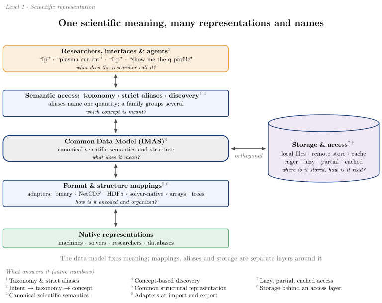
vaft.diagram.scientific_representation()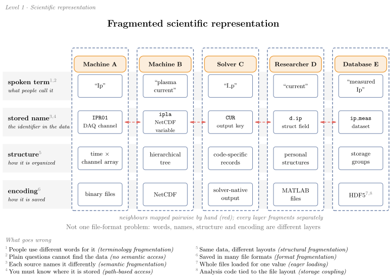
vaft.diagram.scientific_representation(organization='fragmented')Scientific representation, fragmented and layered: one meaning, many representations and names (#1641).
vaft.diagram.scientific_representation(organization='integrated', *, labels=True)Formats .svg .tex .pdf the SVG above is committed; build the others locally
import vaft.diagram
d = vaft.diagram.scientific_representation()
d.tikz # the TikZ document as text
d.save("scientific_representation.svg") # rendered vector image, the canonical artifact; needs latex, dvisvgm
d.save("scientific_representation.tex") # the complete TikZ document, the text source
d.save("scientific_representation.pdf") # vector PDF; needs pdflatexexperimental_research_infrastructure
2 assets
source
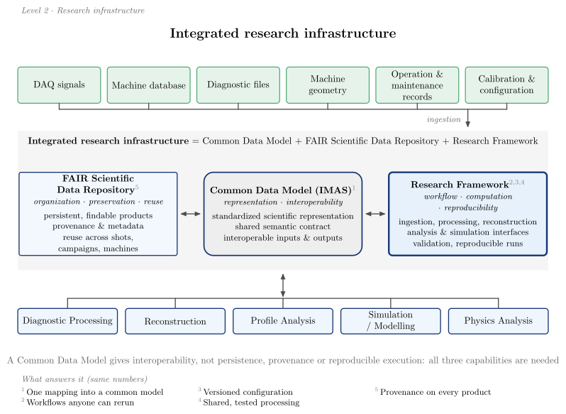
vaft.diagram.experimental_research_infrastructure()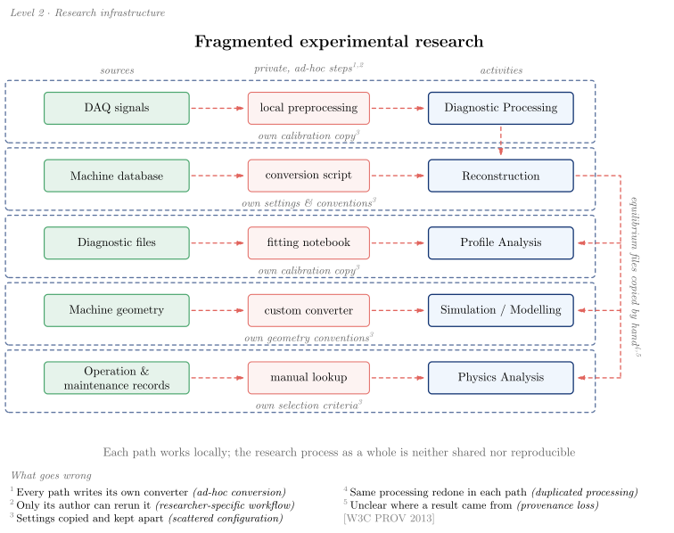
vaft.diagram.experimental_research_infrastructure(organization='fragmented')Experimental research, fragmented and integrated: why a Common Data Model alone is not enough (#1636).
vaft.diagram.experimental_research_infrastructure(organization='integrated', *, labels=True)Formats .svg .tex .pdf the SVG above is committed; build the others locally
import vaft.diagram
d = vaft.diagram.experimental_research_infrastructure()
d.tikz # the TikZ document as text
d.save("experimental_research_infrastructure.svg") # rendered vector image, the canonical artifact; needs latex, dvisvgm
d.save("experimental_research_infrastructure.tex") # the complete TikZ document, the text source
d.save("experimental_research_infrastructure.pdf") # vector PDF; needs pdflatexscientific_credibility
2 assets
source
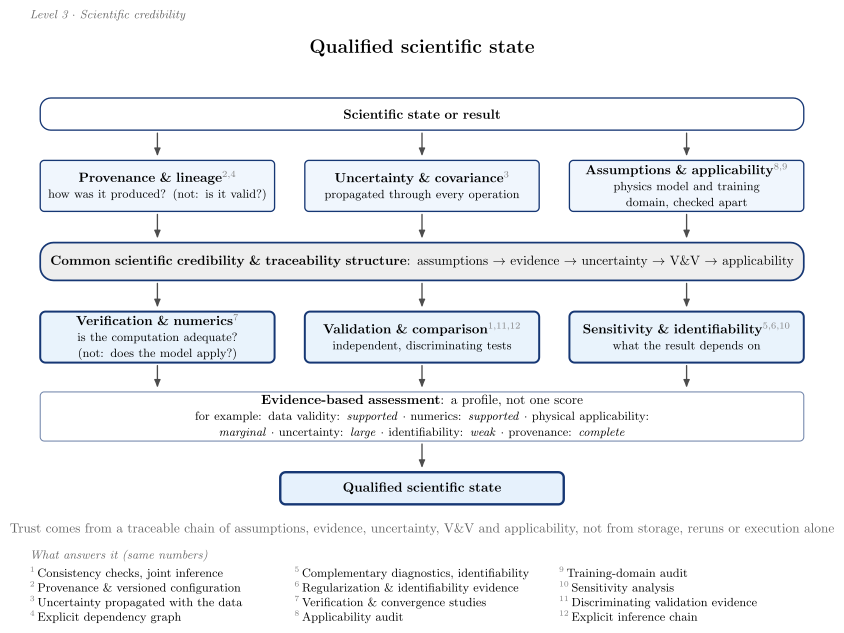
vaft.diagram.scientific_credibility()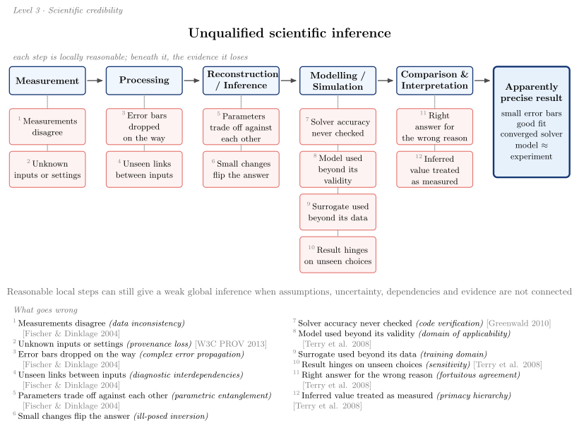
vaft.diagram.scientific_credibility(organization='fragmented')Scientific credibility, fragmented and qualified: why reproducibility is not enough (#1638).
vaft.diagram.scientific_credibility(organization='integrated', *, labels=True)Formats .svg .tex .pdf the SVG above is committed; build the others locally
import vaft.diagram
d = vaft.diagram.scientific_credibility()
d.tikz # the TikZ document as text
d.save("scientific_credibility.svg") # rendered vector image, the canonical artifact; needs latex, dvisvgm
d.save("scientific_credibility.tex") # the complete TikZ document, the text source
d.save("scientific_credibility.pdf") # vector PDF; needs pdflatexresearch_modality_architecture
2 assets
source
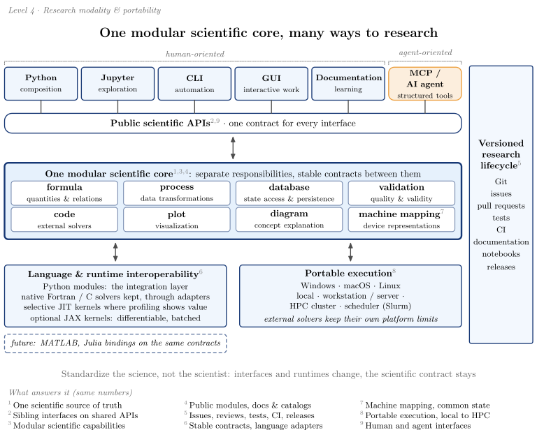
vaft.diagram.research_modality_architecture()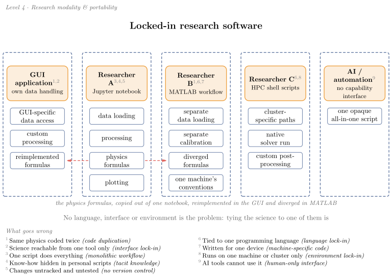
vaft.diagram.research_modality_architecture(organization='fragmented')Research software, locked in and modular: one scientific core, many ways to research (#1640).
vaft.diagram.research_modality_architecture(organization='integrated', *, labels=True)Formats .svg .tex .pdf the SVG above is committed; build the others locally
import vaft.diagram
d = vaft.diagram.research_modality_architecture()
d.tikz # the TikZ document as text
d.save("research_modality_architecture.svg") # rendered vector image, the canonical artifact; needs latex, dvisvgm
d.save("research_modality_architecture.tex") # the complete TikZ document, the text source
d.save("research_modality_architecture.pdf") # vector PDF; needs pdflatexfusion_research_ecosystem
2 assets
source
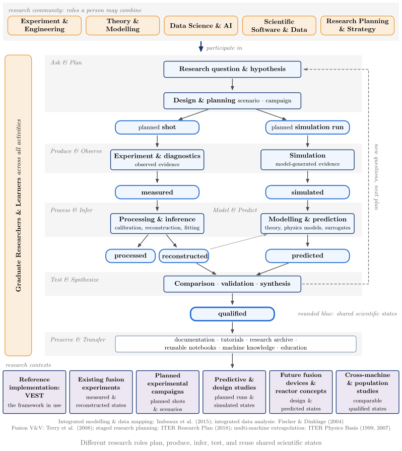
vaft.diagram.fusion_research_ecosystem()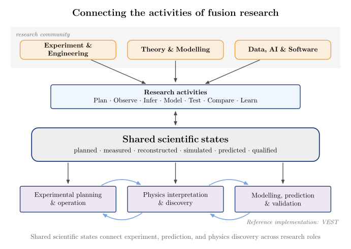
vaft.diagram.fusion_research_ecosystem(detail='presentation')Who does fusion research, what they do, and the shared scientific states that connect it (#1643).
vaft.diagram.fusion_research_ecosystem(detail='full', *, labels=True)Formats .svg .tex .pdf the SVG above is committed; build the others locally
import vaft.diagram
d = vaft.diagram.fusion_research_ecosystem()
d.tikz # the TikZ document as text
d.save("fusion_research_ecosystem.svg") # rendered vector image, the canonical artifact; needs latex, dvisvgm
d.save("fusion_research_ecosystem.tex") # the complete TikZ document, the text source
d.save("fusion_research_ecosystem.pdf") # vector PDF; needs pdflatexscientific_ownership_architecture
1 asset
source
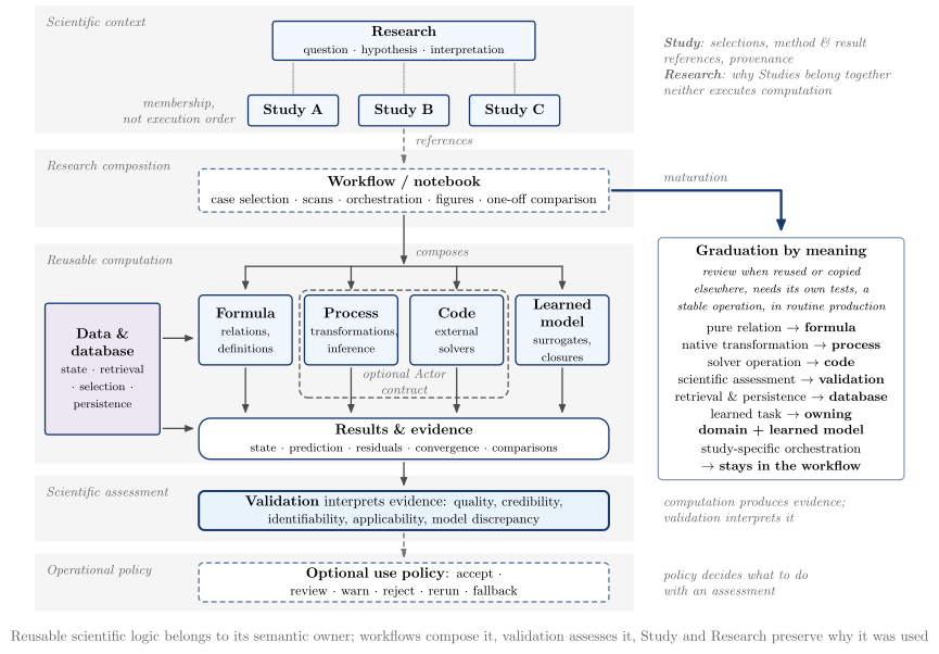
vaft.diagram.scientific_ownership_architecture()Where scientific logic lives as research software matures (#1645).
vaft.diagram.scientific_ownership_architecture(*, labels=True)Formats .svg .tex .pdf the SVG above is committed; build the others locally
import vaft.diagram
d = vaft.diagram.scientific_ownership_architecture()
d.tikz # the TikZ document as text
d.save("scientific_ownership_architecture.svg") # rendered vector image, the canonical artifact; needs latex, dvisvgm
d.save("scientific_ownership_architecture.tex") # the complete TikZ document, the text source
d.save("scientific_ownership_architecture.pdf") # vector PDF; needs pdflatexThe VEST data platform as a database-centred scientific workflow
Module vaft.diagram._platform
vest_data_platform
1 asset
source
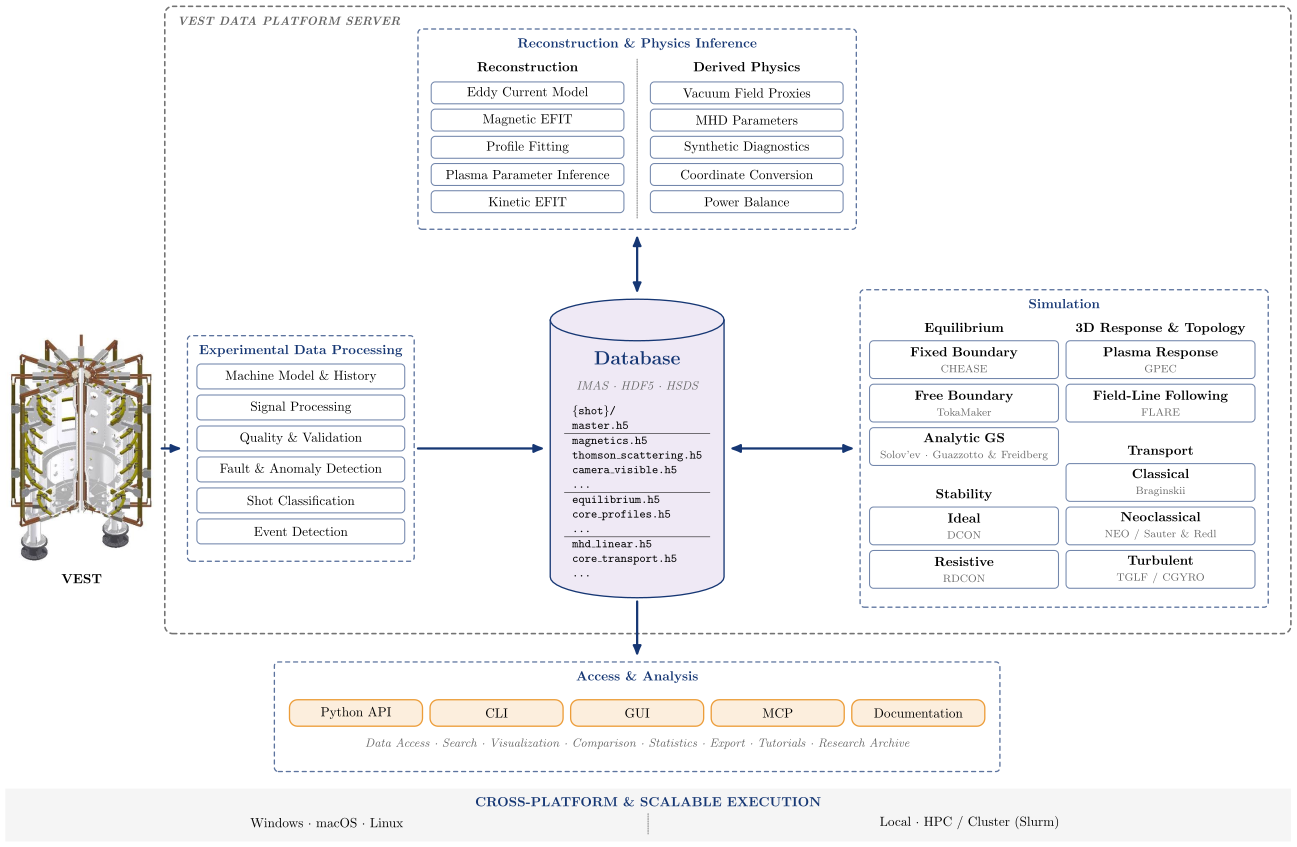
vaft.diagram.vest_data_platform()The VEST data platform: a per-shot database at the centre of experiment, inference and simulation.
vaft.diagram.vest_data_platform(*, labels=True)Formats .svg .tex .pdf the SVG above is committed; build the others locally
import vaft.diagram
d = vaft.diagram.vest_data_platform()
d.tikz # the TikZ document as text
d.save("vest_data_platform.svg") # rendered vector image, the canonical artifact; needs latex, dvisvgm
d.save("vest_data_platform.tex") # the complete TikZ document, the text source
d.save("vest_data_platform.pdf") # vector PDF; needs pdflatexvest_data_platform_overview
1 asset
source
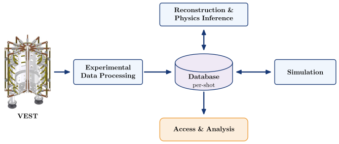
vaft.diagram.vest_data_platform_overview()The VEST data platform in five stages, for papers, slides and introductions.
vaft.diagram.vest_data_platform_overview(*, labels=True)Show source vaft/diagram/_platform.py, lines 306–347
def vest_data_platform_overview(*, labels: bool = True) -> Diagram:
r"""The VEST data platform in five stages, for papers, slides and introductions.
Experiment (the VEST machine) $\to$ experimental data processing $\to$
the per-shot database $\leftrightarrow$ reconstruction and simulation
$\to$ access and analysis. No file contents or sub-items: the
reference view is ``vest_data_platform``.
"""
labels = _check_labels(labels)
items: List = []
machine = _machine(1.4, 0.0, 4.0, items)
proc = _leaf(5.6, 0.0, 3.6, 1.3, _bold("Experimental Data Processing"), "stage:processing", latex=True,
style="concept box")
db = _concept_database(10.6, 0.0, 3.0, 1.9, "\\textbf{Database}\\\\{\\small per-shot}", role="stage:database",
text_style="concept plain", latex=True)
reco = _leaf(10.6, 3.0, 4.6, 1.2, _bold("Reconstruction & Physics Inference"), "stage:reconstruction",
latex=True, style="concept box")
sim = _leaf(15.9, 0.0, 3.2, 1.3, _bold("Simulation"), "stage:simulation", latex=True, style="concept box")
acc = _leaf(10.6, -3.0, 4.6, 1.2, _bold("Access & Analysis"), "stage:access", latex=True,
style="concept actor")
for b in (proc, db, reco, sim, acc):
items += list(b.items)
items += [Arrow((machine[1] + 0.1, 0.0), (proc.x - 0.5 * proc.width - 0.1, 0.0), "connector strong",
role="edge:machine->processing"),
Arrow((proc.x + 0.5 * proc.width + 0.1, 0.0), (db.x - 0.5 * db.width - 0.1, 0.0), "connector strong",
role="edge:processing->database"),
Arrow((db.x, 0.5 * db.height + 0.1), (reco.x, reco.y - 0.5 * reco.height - 0.1), "connector strong",
role="edge:database->reconstruction", both=True),
Arrow((db.x + 0.5 * db.width + 0.1, 0.0), (sim.x - 0.5 * sim.width - 0.1, 0.0), "connector strong",
role="edge:database->simulation", both=True),
Arrow((db.x, -0.5 * db.height - 0.1), (acc.x, acc.y + 0.5 * acc.height + 0.1), "connector strong",
role="edge:database->access")]
edges = (("machine", "processing", "forward"), ("processing", "database", "forward"),
("database", "reconstruction", "both"), ("database", "simulation", "both"),
("database", "access", "forward"))
if labels:
items.append(Label((1.4, machine[2] - 0.05), "\\textbf{VEST}", "concept plain", anchor="north",
role="machine:title"))
else:
items = [it for it in items if not isinstance(it, Label)]
return Diagram("vest_data_platform_overview", Scene(tuple(items)),
model={"edges": edges, "stages": OVERVIEW_STAGES, "machine_extent": machine})Formats .svg .tex .pdf the SVG above is committed; build the others locally
import vaft.diagram
d = vaft.diagram.vest_data_platform_overview()
d.tikz # the TikZ document as text
d.save("vest_data_platform_overview.svg") # rendered vector image, the canonical artifact; needs latex, dvisvgm
d.save("vest_data_platform_overview.tex") # the complete TikZ document, the text source
d.save("vest_data_platform_overview.pdf") # vector PDF; needs pdflatexSoftware dependencies and external scientific-code integration
Module vaft.diagram._ecosystem
software_dependency_ecosystem
1 asset
source
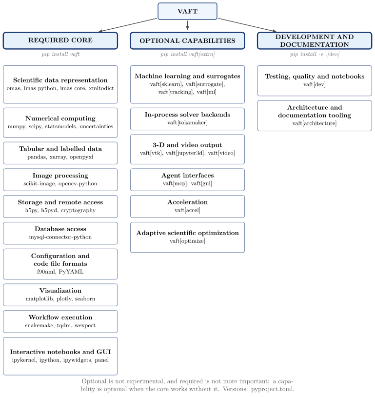
vaft.diagram.software_dependency_ecosystem()Which software capabilities are core, and which an extra or development install activates.
vaft.diagram.software_dependency_ecosystem(*, labels=True)Show source vaft/diagram/_ecosystem.py, lines 65–106
def software_dependency_ecosystem(*, labels: bool = True) -> Diagram:
r"""Which software capabilities are core, and which an extra or development install activates.
VAFT at the top; below it three columns -- the required core, the
optional capabilities, development and documentation -- each listing its
capability roles with the packages (core) or extras (otherwise) that
provide them. Capability is the emphasis, not the package: optional means
only that the core works without it, and packaging status is not a
scientific ranking. Versions are deliberately absent.
"""
labels = _check_labels(labels)
col_w, gap = 6.2, 0.7
xs = [i * (col_w + gap) for i in range(3)]
top = 0.0
root = box(xs[1], top + 1.6, 3.2, 0.9, r"\textbf{VAFT}", role="vaft", latex=True)
items: List = list(root.items)
model: Dict[str, Sequence[str]] = {}
for x, (scope, title, command) in zip(xs, _SCOPES):
head = box(x, top, col_w, 0.9, rf"\textbf{{{escape_latex(title)}}}", style="concept strong",
text_style="concept plain", role=f"scope:{scope}", latex=True)
items += list(head.items) + [connector(root, head, role=f"scope:{scope}")]
if labels:
items.append(Label((x, top - 0.75), command, "concept annotation", role=f"scope:{scope}:install"))
y = top - 1.35
capabilities = [c for c in ecosystem.CAPABILITIES if c.scope == scope]
members = _members(scope)
for capability in capabilities:
listing = ", ".join(members[capability.id])
text = rf"\textbf{{{escape_latex(capability.title)}}}\\{{\small {escape_latex(listing)}}}"
h = _height(capability.title, listing, col_w)
b = box(x, y - 0.5 * h, col_w, h, text, style="concept leaf", text_style="concept plain",
role=f"capability:{capability.id}", latex=True)
items += list(b.items)
y -= h + 0.25
model[scope] = tuple(c.id for c in capabilities)
if labels:
bottom = min(item.at[1] for item in items if isinstance(item, Label)) - 1.1
items.append(Label((xs[1], bottom),
"Optional is not experimental, and required is not more important: a capability is "
"optional when the core works without it. Versions: pyproject.toml.",
"note,text width=18cm", anchor="north", role="note"))
return Diagram("software_dependency_ecosystem", Scene(tuple(items)), model=dict(model))Formats .svg .tex .pdf the SVG above is committed; build the others locally
import vaft.diagram
d = vaft.diagram.software_dependency_ecosystem()
d.tikz # the TikZ document as text
d.save("software_dependency_ecosystem.svg") # rendered vector image, the canonical artifact; needs latex, dvisvgm
d.save("software_dependency_ecosystem.tex") # the complete TikZ document, the text source
d.save("software_dependency_ecosystem.pdf") # vector PDF; needs pdflatexexternal_code_integration
1 asset
source
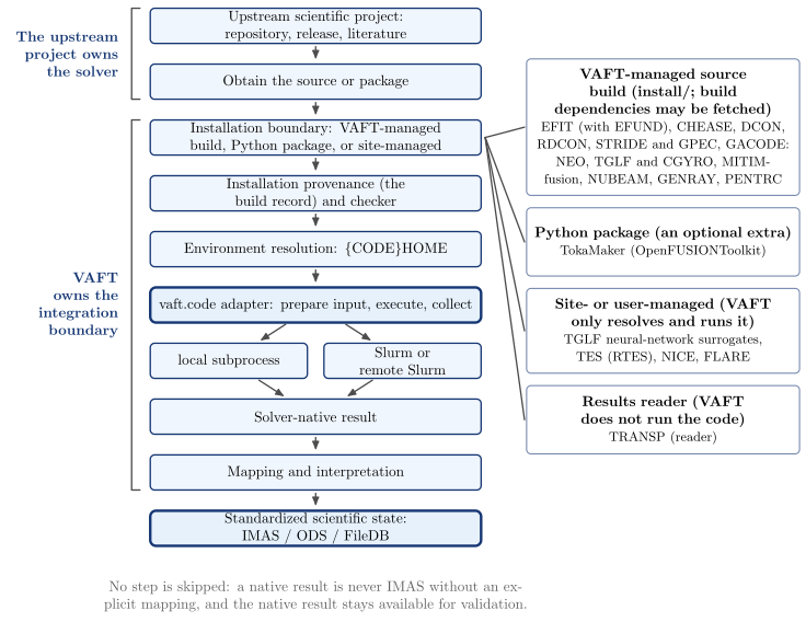
vaft.diagram.external_code_integration()How an independently maintained scientific code becomes a reproducible VAFT capability.
vaft.diagram.external_code_integration(*, labels=True)Show source vaft/diagram/_ecosystem.py, lines 109–180
def external_code_integration(*, labels: bool = True) -> Diagram:
r"""How an independently maintained scientific code becomes a reproducible VAFT capability.
The integration lifecycle top to bottom: the upstream project, obtaining
its source or package, the installation boundary, installation
provenance and checker, ``{CODE}HOME`` resolution, the ``vaft.code``
adapter, local or scheduler-backed execution, the solver-native result,
mapping, and the standardized IMAS/ODS/FileDB state. The upstream
project owns the solver; VAFT owns the integration boundary. Beside the
installation step, the current codes grouped by who installs them.
"""
labels = _check_labels(labels)
w, h, step = 8.0, 0.85, 1.35
boxes = {}
items: List = []
y = 0.0
for key, text in ecosystem.INTEGRATION_LIFECYCLE:
if key == "execute":
local = box(-2.1, y, 3.8, h, "local subprocess", text_style="concept plain", role="lifecycle:execute:local")
hpc = box(2.1, y, 3.8, h, "Slurm or remote Slurm", text_style="concept plain",
role="lifecycle:execute:slurm")
items += list(local.items) + list(hpc.items)
boxes[key] = (local, hpc)
else:
style = "concept strong" if key in {"adapter", "standard"} else "concept box"
b = box(0.0, y, w, h, text, style=style, text_style="concept plain", role=f"lifecycle:{key}")
items += list(b.items)
boxes[key] = (b,)
y -= step
keys = [key for key, _ in ecosystem.INTEGRATION_LIFECYCLE]
for upper, lower in zip(keys, keys[1:]):
for a in boxes[upper]:
for b in boxes[lower]:
items.append(connector(a, b, role=f"flow:{upper}->{lower}"))
# ownership brackets on the left
def bracket(first: str, last: str, text: str, role: str) -> None:
y0 = boxes[first][0].y + 0.5 * h
y1 = boxes[last][0].y - 0.5 * h
x = -0.5 * w - 0.45
items.append(Polyline.of([(x + 0.2, y0), (x, y0), (x, y1), (x + 0.2, y1)], "connector line", role=role))
items.append(Label((x - 0.2, 0.5 * (y0 + y1)), text, "concept group title,text width=2.6cm,align=right,"
"execute at begin node={\\hyphenpenalty=10000}",
anchor="east", role=role))
bracket("upstream", "obtain", "The upstream project owns the solver", "owner:upstream")
bracket("install", "mapping", "VAFT owns the integration boundary", "owner:vaft")
# the codes, by who installs them
install = boxes["install"][0]
side_x = 0.5 * w + 4.4
groups: Dict[str, List[str]] = {}
for code in ecosystem.EXTERNAL_CODES:
groups.setdefault(code.installation, []).append(code.name)
gy = install.y + 1.9
for installation in ("vaft_managed_source_build", "python_package", "site_managed", "reader_only"):
names = groups.get(installation, [])
if not names:
continue
text = (rf"\textbf{{{escape_latex(_INSTALLATION_TITLES[installation])}}}\\"
rf"{{\small {escape_latex(', '.join(names))}}}")
bh = _height(_INSTALLATION_TITLES[installation], ", ".join(names), 6.6)
g = box(side_x, gy - 0.5 * bh, 6.6, bh, text, style="concept leaf", text_style="concept plain",
role=f"installation:{installation}", latex=True)
items += list(g.items)
items.append(Arrow((side_x - 3.35, gy - 0.5 * bh), (0.5 * w + 0.1, install.y), "connector line",
role=f"installation:{installation}"))
gy -= bh + 0.3
if labels:
items.append(Label((0.0, y + 0.2), "No step is skipped: a native result is never IMAS without an explicit "
"mapping, and the native result stays available for validation.",
"note,text width=14cm", anchor="north", role="note"))
model = {"lifecycle": tuple(keys),
"installation": {k: tuple(v) for k, v in sorted(groups.items())}}
return Diagram("external_code_integration", Scene(tuple(items)), model=model)Formats .svg .tex .pdf the SVG above is committed; build the others locally
import vaft.diagram
d = vaft.diagram.external_code_integration()
d.tikz # the TikZ document as text
d.save("external_code_integration.svg") # rendered vector image, the canonical artifact; needs latex, dvisvgm
d.save("external_code_integration.tex") # the complete TikZ document, the text source
d.save("external_code_integration.pdf") # vector PDF; needs pdflatexThe state-to-simulation spine (#1585): physics workflows from measured state to standardized IMAS results
Module vaft.diagram._workflow_specs
plasma_parameter_inference
1 asset
source
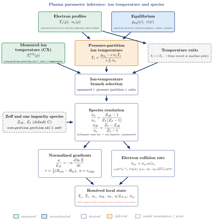
vaft.diagram.plasma_parameter_inference()Electron profiles and the equilibrium resolved into T_i, the species mix and the local state.
vaft.diagram.plasma_parameter_inference(*, labels=True)Show source vaft/diagram/_workflow_specs.py, lines 584–586
def plasma_parameter_inference(*, labels: bool = True) -> Diagram:
"""Electron profiles and the equilibrium resolved into T_i, the species mix and the local state."""
return _render_workflow(WORKFLOWS["plasma_parameter_inference"], labels=labels)Formats .svg .tex .pdf the SVG above is committed; build the others locally
import vaft.diagram
d = vaft.diagram.plasma_parameter_inference()
d.tikz # the TikZ document as text
d.save("plasma_parameter_inference.svg") # rendered vector image, the canonical artifact; needs latex, dvisvgm
d.save("plasma_parameter_inference.tex") # the complete TikZ document, the text source
d.save("plasma_parameter_inference.pdf") # vector PDF; needs pdflatexromero_transformer_balance
1 asset
source
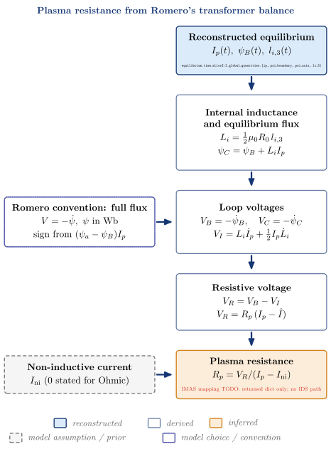
vaft.diagram.romero_transformer_balance()Plasma resistance from Romero’s exact transformer balance.
vaft.diagram.romero_transformer_balance(*, labels=True)Show source vaft/diagram/_workflow_specs.py, lines 589–591
def romero_transformer_balance(*, labels: bool = True) -> Diagram:
"""Plasma resistance from Romero's exact transformer balance."""
return _render_workflow(WORKFLOWS["romero_transformer_balance"], labels=labels)Formats .svg .tex .pdf the SVG above is committed; build the others locally
import vaft.diagram
d = vaft.diagram.romero_transformer_balance()
d.tikz # the TikZ document as text
d.save("romero_transformer_balance.svg") # rendered vector image, the canonical artifact; needs latex, dvisvgm
d.save("romero_transformer_balance.tex") # the complete TikZ document, the text source
d.save("romero_transformer_balance.pdf") # vector PDF; needs pdflatexresistive_zeff_inference
1 asset
source
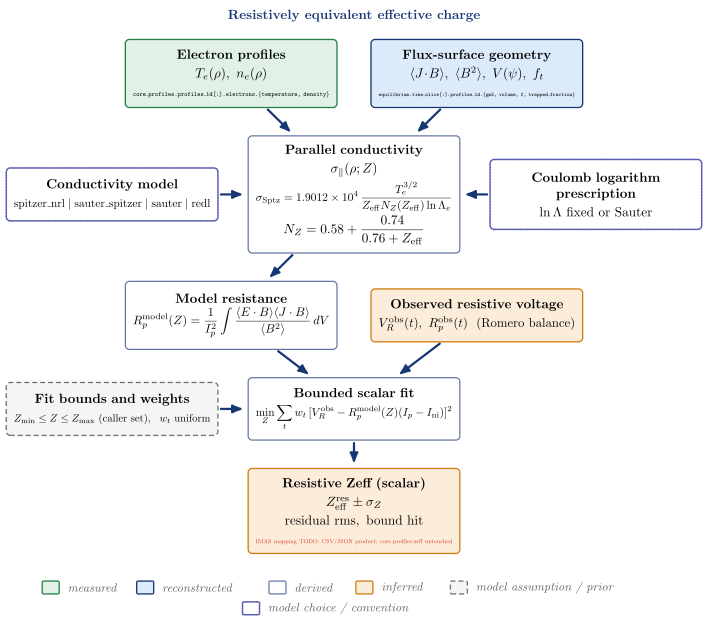
vaft.diagram.resistive_zeff_inference()The resistively equivalent scalar Zeff a conductivity model needs to match the observed resistance.
vaft.diagram.resistive_zeff_inference(*, labels=True)Show source vaft/diagram/_workflow_specs.py, lines 594–596
def resistive_zeff_inference(*, labels: bool = True) -> Diagram:
"""The resistively equivalent scalar Zeff a conductivity model needs to match the observed resistance."""
return _render_workflow(WORKFLOWS["resistive_zeff_inference"], labels=labels)Formats .svg .tex .pdf the SVG above is committed; build the others locally
import vaft.diagram
d = vaft.diagram.resistive_zeff_inference()
d.tikz # the TikZ document as text
d.save("resistive_zeff_inference.svg") # rendered vector image, the canonical artifact; needs latex, dvisvgm
d.save("resistive_zeff_inference.tex") # the complete TikZ document, the text source
d.save("resistive_zeff_inference.pdf") # vector PDF; needs pdflatexmagnetic_efit
1 asset
source
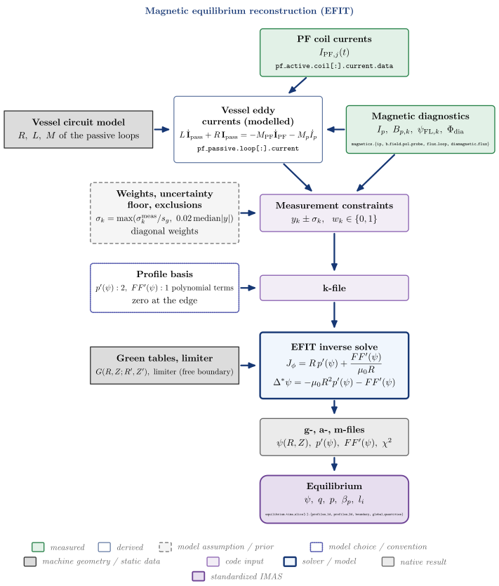
vaft.diagram.magnetic_efit()Magnetic equilibrium reconstruction: a free-boundary inverse problem.
vaft.diagram.magnetic_efit(*, labels=True)Show source vaft/diagram/_workflow_specs.py, lines 599–601
def magnetic_efit(*, labels: bool = True) -> Diagram:
"""Magnetic equilibrium reconstruction: a free-boundary inverse problem."""
return _render_workflow(WORKFLOWS["magnetic_efit"], labels=labels)Formats .svg .tex .pdf the SVG above is committed; build the others locally
import vaft.diagram
d = vaft.diagram.magnetic_efit()
d.tikz # the TikZ document as text
d.save("magnetic_efit.svg") # rendered vector image, the canonical artifact; needs latex, dvisvgm
d.save("magnetic_efit.tex") # the complete TikZ document, the text source
d.save("magnetic_efit.pdf") # vector PDF; needs pdflatexkinetic_efit
1 asset
source
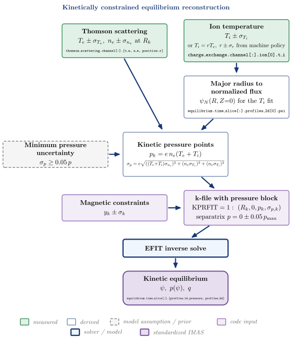
vaft.diagram.kinetic_efit()Kinetically constrained reconstruction: magnetic constraints plus kinetic pressure points.
vaft.diagram.kinetic_efit(*, labels=True)Show source vaft/diagram/_workflow_specs.py, lines 604–606
def kinetic_efit(*, labels: bool = True) -> Diagram:
"""Kinetically constrained reconstruction: magnetic constraints plus kinetic pressure points."""
return _render_workflow(WORKFLOWS["kinetic_efit"], labels=labels)Formats .svg .tex .pdf the SVG above is committed; build the others locally
import vaft.diagram
d = vaft.diagram.kinetic_efit()
d.tikz # the TikZ document as text
d.save("kinetic_efit.svg") # rendered vector image, the canonical artifact; needs latex, dvisvgm
d.save("kinetic_efit.tex") # the complete TikZ document, the text source
d.save("kinetic_efit.pdf") # vector PDF; needs pdflatexanalytic_mhd_equilibrium
1 asset
source
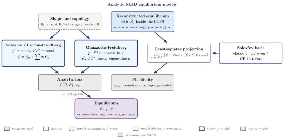
vaft.diagram.analytic_mhd_equilibrium()Analytic MHD equilibria: forward generation and projection onto a Solov’ev basis.
vaft.diagram.analytic_mhd_equilibrium(*, labels=True)Show source vaft/diagram/_workflow_specs.py, lines 609–611
def analytic_mhd_equilibrium(*, labels: bool = True) -> Diagram:
"""Analytic MHD equilibria: forward generation and projection onto a Solov'ev basis."""
return _render_workflow(WORKFLOWS["analytic_mhd_equilibrium"], labels=labels)Formats .svg .tex .pdf the SVG above is committed; build the others locally
import vaft.diagram
d = vaft.diagram.analytic_mhd_equilibrium()
d.tikz # the TikZ document as text
d.save("analytic_mhd_equilibrium.svg") # rendered vector image, the canonical artifact; needs latex, dvisvgm
d.save("analytic_mhd_equilibrium.tex") # the complete TikZ document, the text source
d.save("analytic_mhd_equilibrium.pdf") # vector PDF; needs pdflatexchease_coupling
1 asset
source
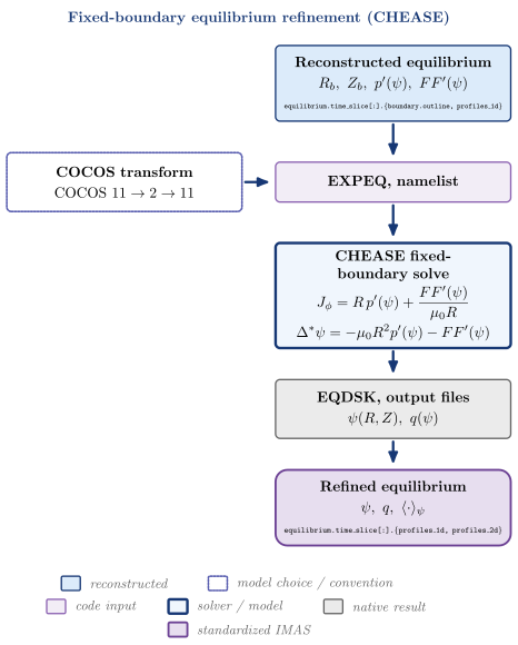
vaft.diagram.chease_coupling()Fixed-boundary refinement with CHEASE, COCOS transform explicit.
vaft.diagram.chease_coupling(*, labels=True)Show source vaft/diagram/_workflow_specs.py, lines 614–616
def chease_coupling(*, labels: bool = True) -> Diagram:
"""Fixed-boundary refinement with CHEASE, COCOS transform explicit."""
return _render_workflow(WORKFLOWS["chease_coupling"], labels=labels)Formats .svg .tex .pdf the SVG above is committed; build the others locally
import vaft.diagram
d = vaft.diagram.chease_coupling()
d.tikz # the TikZ document as text
d.save("chease_coupling.svg") # rendered vector image, the canonical artifact; needs latex, dvisvgm
d.save("chease_coupling.tex") # the complete TikZ document, the text source
d.save("chease_coupling.pdf") # vector PDF; needs pdflatextokamaker_coupling
1 asset
source
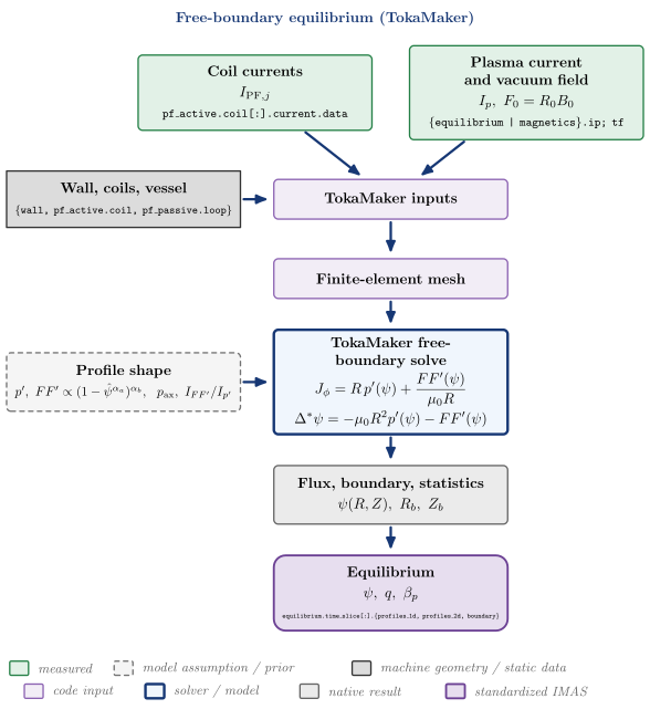
vaft.diagram.tokamaker_coupling()Free-boundary equilibrium with TokaMaker.
vaft.diagram.tokamaker_coupling(*, labels=True)Show source vaft/diagram/_workflow_specs.py, lines 619–621
def tokamaker_coupling(*, labels: bool = True) -> Diagram:
"""Free-boundary equilibrium with TokaMaker."""
return _render_workflow(WORKFLOWS["tokamaker_coupling"], labels=labels)Formats .svg .tex .pdf the SVG above is committed; build the others locally
import vaft.diagram
d = vaft.diagram.tokamaker_coupling()
d.tikz # the TikZ document as text
d.save("tokamaker_coupling.svg") # rendered vector image, the canonical artifact; needs latex, dvisvgm
d.save("tokamaker_coupling.tex") # the complete TikZ document, the text source
d.save("tokamaker_coupling.pdf") # vector PDF; needs pdflatexdcon_rdcon_stability
1 asset
source
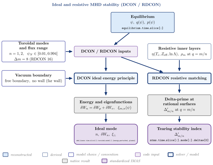
vaft.diagram.dcon_rdcon_stability()Ideal and resistive MHD stability with DCON and RDCON.
vaft.diagram.dcon_rdcon_stability(*, labels=True)Show source vaft/diagram/_workflow_specs.py, lines 624–626
def dcon_rdcon_stability(*, labels: bool = True) -> Diagram:
"""Ideal and resistive MHD stability with DCON and RDCON."""
return _render_workflow(WORKFLOWS["dcon_rdcon_stability"], labels=labels)Formats .svg .tex .pdf the SVG above is committed; build the others locally
import vaft.diagram
d = vaft.diagram.dcon_rdcon_stability()
d.tikz # the TikZ document as text
d.save("dcon_rdcon_stability.svg") # rendered vector image, the canonical artifact; needs latex, dvisvgm
d.save("dcon_rdcon_stability.tex") # the complete TikZ document, the text source
d.save("dcon_rdcon_stability.pdf") # vector PDF; needs pdflatexgpec_plasma_response
1 asset
source
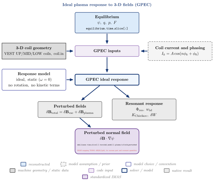
vaft.diagram.gpec_plasma_response()The ideal plasma response to applied 3-D fields with GPEC.
vaft.diagram.gpec_plasma_response(*, labels=True)Show source vaft/diagram/_workflow_specs.py, lines 629–631
def gpec_plasma_response(*, labels: bool = True) -> Diagram:
"""The ideal plasma response to applied 3-D fields with GPEC."""
return _render_workflow(WORKFLOWS["gpec_plasma_response"], labels=labels)Formats .svg .tex .pdf the SVG above is committed; build the others locally
import vaft.diagram
d = vaft.diagram.gpec_plasma_response()
d.tikz # the TikZ document as text
d.save("gpec_plasma_response.svg") # rendered vector image, the canonical artifact; needs latex, dvisvgm
d.save("gpec_plasma_response.tex") # the complete TikZ document, the text source
d.save("gpec_plasma_response.pdf") # vector PDF; needs pdflatexflare_field_line_topology
1 asset
source
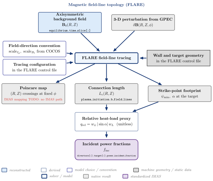
vaft.diagram.flare_field_line_topology()Magnetic field-line topology with FLARE.
vaft.diagram.flare_field_line_topology(*, labels=True)Show source vaft/diagram/_workflow_specs.py, lines 634–636
def flare_field_line_topology(*, labels: bool = True) -> Diagram:
"""Magnetic field-line topology with FLARE."""
return _render_workflow(WORKFLOWS["flare_field_line_topology"], labels=labels)Formats .svg .tex .pdf the SVG above is committed; build the others locally
import vaft.diagram
d = vaft.diagram.flare_field_line_topology()
d.tikz # the TikZ document as text
d.save("flare_field_line_topology.svg") # rendered vector image, the canonical artifact; needs latex, dvisvgm
d.save("flare_field_line_topology.tex") # the complete TikZ document, the text source
d.save("flare_field_line_topology.pdf") # vector PDF; needs pdflatexneo_neoclassical
1 asset
source
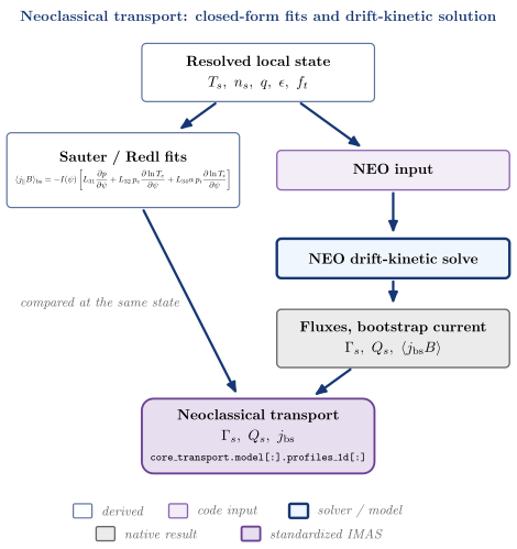
vaft.diagram.neo_neoclassical()Neoclassical transport: Sauter / Redl fits and NEO at one state.
vaft.diagram.neo_neoclassical(*, labels=True)Show source vaft/diagram/_workflow_specs.py, lines 639–641
def neo_neoclassical(*, labels: bool = True) -> Diagram:
"""Neoclassical transport: Sauter / Redl fits and NEO at one state."""
return _render_workflow(WORKFLOWS["neo_neoclassical"], labels=labels)Formats .svg .tex .pdf the SVG above is committed; build the others locally
import vaft.diagram
d = vaft.diagram.neo_neoclassical()
d.tikz # the TikZ document as text
d.save("neo_neoclassical.svg") # rendered vector image, the canonical artifact; needs latex, dvisvgm
d.save("neo_neoclassical.tex") # the complete TikZ document, the text source
d.save("neo_neoclassical.pdf") # vector PDF; needs pdflatextglf_cgyro_local_transport
1 asset
source
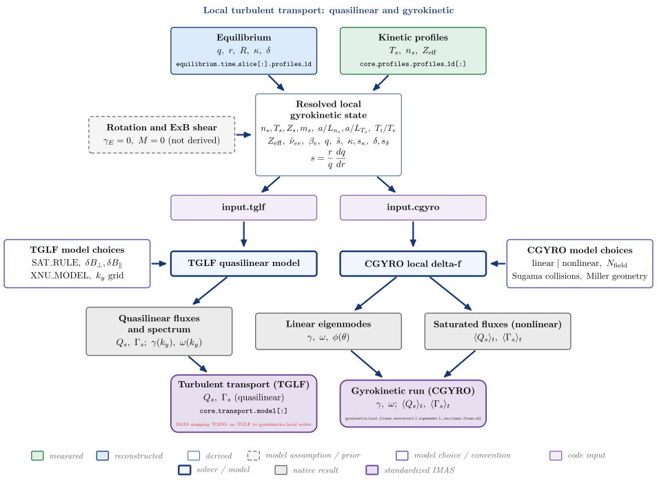
vaft.diagram.tglf_cgyro_local_transport()Local turbulent transport: TGLF and CGYRO from one local state.
vaft.diagram.tglf_cgyro_local_transport(*, labels=True)Show source vaft/diagram/_workflow_specs.py, lines 644–646
def tglf_cgyro_local_transport(*, labels: bool = True) -> Diagram:
"""Local turbulent transport: TGLF and CGYRO from one local state."""
return _render_workflow(WORKFLOWS["tglf_cgyro_local_transport"], labels=labels)Formats .svg .tex .pdf the SVG above is committed; build the others locally
import vaft.diagram
d = vaft.diagram.tglf_cgyro_local_transport()
d.tikz # the TikZ document as text
d.save("tglf_cgyro_local_transport.svg") # rendered vector image, the canonical artifact; needs latex, dvisvgm
d.save("tglf_cgyro_local_transport.tex") # the complete TikZ document, the text source
d.save("tglf_cgyro_local_transport.pdf") # vector PDF; needs pdflatexparameter_inference_overview
1 asset
source
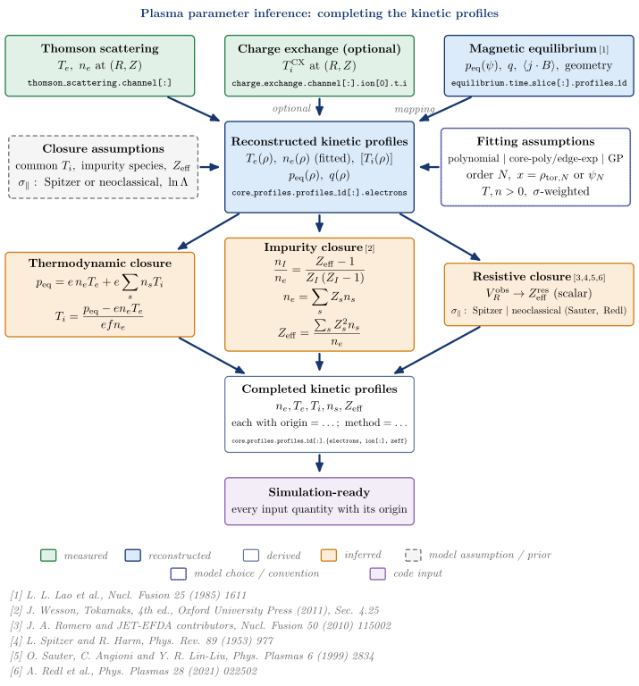
vaft.diagram.parameter_inference_overview(references=True)Where plasma parameter inference sits between reconstruction and simulation (#1601).
vaft.diagram.parameter_inference_overview(*, labels=True, references=False)Show source vaft/diagram/_workflow_specs.py, lines 649–654
def parameter_inference_overview(*, labels: bool = True, references: bool = False) -> Diagram:
"""Where plasma parameter inference sits between reconstruction and simulation (#1601).
``references=True`` numbers each closure's representative papers and lists them under the legend.
"""
return _render_workflow(WORKFLOWS["parameter_inference_overview"], labels=labels, references=references)Formats .svg .tex .pdf the SVG above is committed; build the others locally
import vaft.diagram
d = vaft.diagram.parameter_inference_overview(references=True)
d.tikz # the TikZ document as text
d.save("parameter_inference_overview.svg") # rendered vector image, the canonical artifact; needs latex, dvisvgm
d.save("parameter_inference_overview.tex") # the complete TikZ document, the text source
d.save("parameter_inference_overview.pdf") # vector PDF; needs pdflatexparameter_inference_dependency_graph
1 asset
source
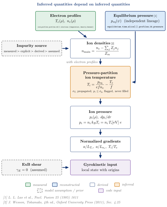
vaft.diagram.parameter_inference_dependency_graph(references=True)How provenance propagates through inferred plasma parameters (#1601).
vaft.diagram.parameter_inference_dependency_graph(*, labels=True, references=False)Show source vaft/diagram/_workflow_specs.py, lines 657–662
def parameter_inference_dependency_graph(*, labels: bool = True, references: bool = False) -> Diagram:
"""How provenance propagates through inferred plasma parameters (#1601).
``references=True`` numbers the representative papers and lists them under the legend.
"""
return _render_workflow(WORKFLOWS["parameter_inference_dependency_graph"], labels=labels, references=references)Formats .svg .tex .pdf the SVG above is committed; build the others locally
import vaft.diagram
d = vaft.diagram.parameter_inference_dependency_graph(references=True)
d.tikz # the TikZ document as text
d.save("parameter_inference_dependency_graph.svg") # rendered vector image, the canonical artifact; needs latex, dvisvgm
d.save("parameter_inference_dependency_graph.tex") # the complete TikZ document, the text source
d.save("parameter_inference_dependency_graph.pdf") # vector PDF; needs pdflatexCoordinates, geometry, meshes, mappings and topology: the spatial vocabulary
Module vaft.diagram._spatial
tokamak_top_view
1 asset
source
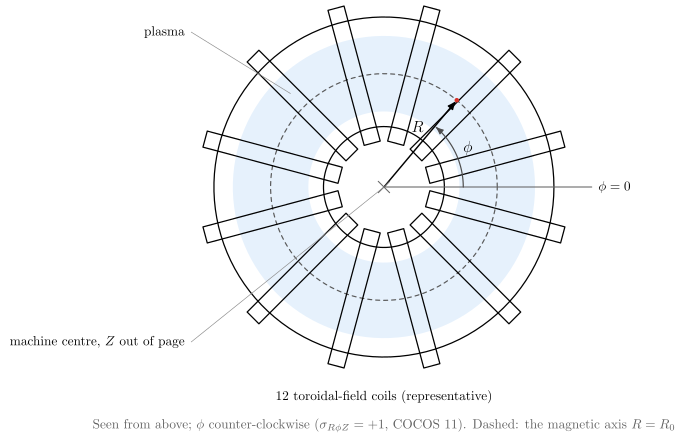
vaft.diagram.tokamak_top_view()The torus seen from above: machine centre, major radius $R$ and toroidal angle $\phi$.
vaft.diagram.tokamak_top_view(*, cocos=11, n_coils=12, labels=True)Show source vaft/diagram/_spatial.py, lines 99–155
def tokamak_top_view(*, cocos: int = 11, n_coils: int = 12, labels: bool = True) -> Diagram:
r"""The torus seen from above: machine centre, major radius $R$ and toroidal angle $\phi$.
The plasma is the annulus $R_0 - a < R < R_0 + a$, the vessel the two
circles around it and the ``n_coils`` toroidal-field coils cross it
radially. $\phi$ is measured from the reference ray $\phi = 0$; its sense
comes from ``cocos`` ($\sigma_{R\phi Z} = +1$: counter-clockwise seen from
above, with $Z$ towards the reader). Representative, not any machine.
"""
labels = _check_labels(labels)
n_coils = _index(n_coils, "n_coils")
if not 4 <= n_coils <= 24:
raise ValueError(f"n_coils must be an integer from 4 to 24, not {n_coils!r}")
cocos = _index(cocos, "cocos")
spec = cocos_spec(cocos)
ccw = _phi_counterclockwise_from_above(spec)
R0, a, r_in, r_out = 3.0, 1.0, 1.6, 4.5
items: List = [Polyline.of(_circle(0, 0, R0 + a), "region plasma", role="plasma", closed=True),
Polyline.of(_circle(0, 0, R0 - a), "hole", role="plasma", closed=True)]
for r in (r_in, r_out):
items.append(Polyline.of(_circle(0, 0, r), "machine", role="vessel", closed=True))
items.append(Polyline.of(_circle(0, 0, R0), "approx", role="magnetic_axis_circle", closed=True))
w = 0.22
for k in range(n_coils):
t = 2.0 * math.pi * (k + 0.5) / n_coils
c, s = math.cos(t), math.sin(t)
corners = [(r * c - h * s, r * s + h * c) for r, h in ((r_in - 0.4, -w), (r_out + 0.4, -w),
(r_out + 0.4, w), (r_in - 0.4, w))]
items.append(Polyline.of(corners, "machine", role="tf_coil", closed=True))
phi_point = math.radians(50.0) * (1 if ccw else -1)
items += [Polyline.of([(0, 0), (r_out + 1.0, 0)], "frame axis", role="phi_reference"),
Arrow((0, 0), (R0 * math.cos(phi_point), R0 * math.sin(phi_point)), "vector", role="major_radius"),
Polyline.of(_circle(0, 0, 2.1, 40, 0.0, phi_point), "angle arc", role="toroidal_angle"),
Marker((R0 * math.cos(phi_point), R0 * math.sin(phi_point)), "o", "diagnostic point", role="point"),
Polyline.of([(-0.15, -0.15), (0.15, 0.15)], "frame axis", role="centre"),
Polyline.of([(-0.15, 0.15), (0.15, -0.15)], "frame axis", role="centre")]
if labels:
mid = 0.5 * phi_point
items += [Label((2.45 * math.cos(mid), 2.45 * math.sin(mid)), "$\\phi$", "label", role="toroidal_angle"),
Label((0.6 * R0 * math.cos(phi_point) - 0.35 * math.sin(phi_point),
0.6 * R0 * math.sin(phi_point) + 0.35 * math.cos(phi_point)), "$R$", "label",
role="major_radius"),
Label((r_out + 1.05, 0), "$\\phi = 0$", "small label", anchor="west", role="phi_reference"),
Polyline.of([(0, 0), (-r_out - 0.6, -r_out + 0.4)], "leader line", role="leader:centre"),
Label((-r_out - 0.65, -r_out + 0.4), "machine centre, $Z$ out of page", "small label",
anchor="east", role="centre"),
Polyline.of([(-(R0 + 0.5) * 0.7071, (R0 + 0.5) * 0.7071), (-r_out - 0.6, r_out - 0.4)],
"leader line", role="leader:plasma"),
Label((-r_out - 0.65, r_out - 0.4), "plasma", "small label", anchor="east", role="plasma"),
Label((0, -r_out - 0.75), f"{n_coils} toroidal-field coils (representative)", "small label",
anchor="north", role="tf_coil"),
_note(f"Seen from above; $\\phi$ {'counter-clockwise' if ccw else 'clockwise'} "
f"($\\sigma_{{R\\phi Z}} = {spec.sigma_rpz:+d}$, COCOS {cocos}). "
"Dashed: the magnetic axis $R = R_0$", 0.0, -r_out - 1.5)]
return Diagram("tokamak_top_view", Scene(tuple(items)),
model={"cocos": cocos, "phi_counterclockwise_from_above": ccw, "n_coils": n_coils,
"phi_point": phi_point})Formats .svg .tex .pdf the SVG above is committed; build the others locally
import vaft.diagram
d = vaft.diagram.tokamak_top_view()
d.tikz # the TikZ document as text
d.save("tokamak_top_view.svg") # rendered vector image, the canonical artifact; needs latex, dvisvgm
d.save("tokamak_top_view.tex") # the complete TikZ document, the text source
d.save("tokamak_top_view.pdf") # vector PDF; needs pdflatexcocos_orientation
2 assets
source
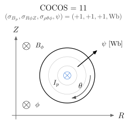
vaft.diagram.cocos_orientation()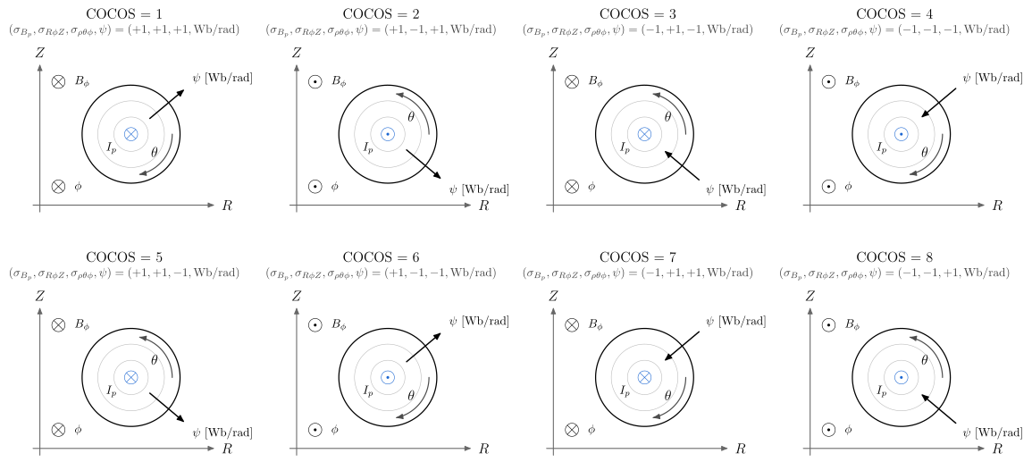
vaft.diagram.cocos_orientation(cocos=(1, 2, 3, 4, 5, 6, 7, 8))What a COCOS index fixes, on a generic poloidal cross-section: one panel per index.
vaft.diagram.cocos_orientation(cocos=11, *, sigma_ip=1, sigma_b0=1, labels=True)Show source vaft/diagram/_spatial.py, lines 231–267
def cocos_orientation(cocos=11, *, sigma_ip: int = 1, sigma_b0: int = 1, labels: bool = True) -> Diagram:
r"""What a COCOS index fixes, on a generic poloidal cross-section: one panel per index.
``cocos`` is one index or a sequence of them, drawn as panels in rows of
four at one scale. In each panel $R$ points right and $Z$ up;
$\odot$/$\otimes$ say whether $\phi$, the toroidal field and the plasma
current (the blue symbol on the magnetic axis) point out of or into the
page; the arc is
the sense of $\theta$; the arrow points where $\psi$ increases and carries
its unit (Wb for full flux, $e_{B_p} = 1$; Wb/rad per radian). Title and
subtitle give the index and
$(\sigma_{B_p}, \sigma_{R\phi Z}, \sigma_{\rho\theta\phi}, \psi)$.
``sigma_ip`` and ``sigma_b0`` are the signs along $\phi$
(:func:`cocos_orientation_signs`; Sauter and Medvedev,
Comput. Phys. Commun. 184 (2013) 293). ``Diagram.model["panels"]`` holds
the signs of every panel.
"""
labels = _check_labels(labels)
if isinstance(cocos, (str, bytes)):
raise ValueError(f"cocos must be an index or a non-empty sequence of indices, not {cocos!r}")
try:
indices = (_index(cocos, "cocos"),)
except ValueError:
if isinstance(cocos, bool):
raise
try:
indices = tuple(_index(i, "cocos") for i in cocos)
except TypeError:
raise ValueError(f"cocos must be an index or a non-empty sequence of indices, not {cocos!r}") from None
if not indices:
raise ValueError(f"cocos must be an index or a non-empty sequence of indices, not {cocos!r}")
signs = tuple(cocos_orientation_signs(i, sigma_ip=sigma_ip, sigma_b0=sigma_b0) for i in indices)
items: List = []
for k, s in enumerate(signs):
row, col = divmod(k, _COCOS_PER_ROW)
items += _cocos_panel(s, (col * _COCOS_DX, -row * _COCOS_DY), labels)
return Diagram("cocos_orientation", Scene(tuple(items)), model={"panels": signs})Formats .svg .tex .pdf the SVG above is committed; build the others locally
import vaft.diagram
d = vaft.diagram.cocos_orientation()
d.tikz # the TikZ document as text
d.save("cocos_orientation.svg") # rendered vector image, the canonical artifact; needs latex, dvisvgm
d.save("cocos_orientation.tex") # the complete TikZ document, the text source
d.save("cocos_orientation.pdf") # vector PDF; needs pdflatexmachine_and_equilibrium_geometry
1 asset
source
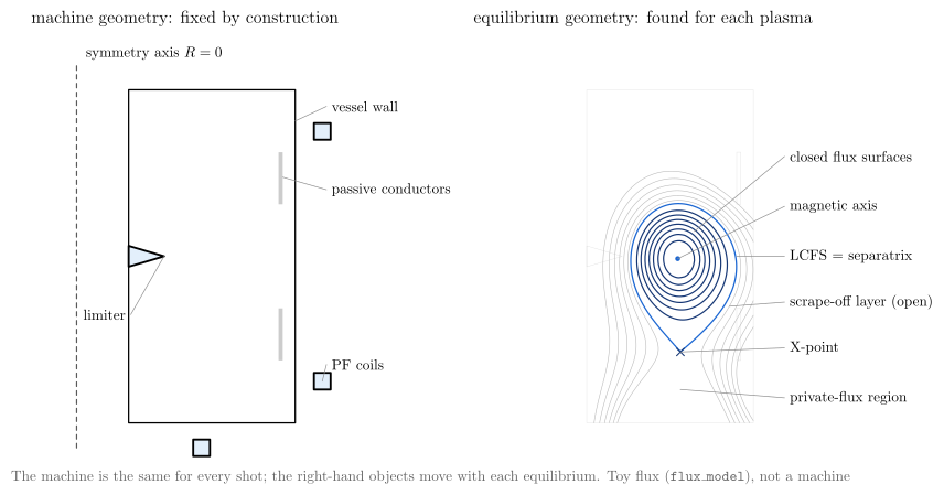
vaft.diagram.machine_and_equilibrium_geometry()Machine geometry against equilibrium geometry: built objects against found ones.
vaft.diagram.machine_and_equilibrium_geometry(*, labels=True)Show source vaft/diagram/_spatial.py, lines 302–354
def machine_and_equilibrium_geometry(*, labels: bool = True) -> Diagram:
r"""Machine geometry against equilibrium geometry: built objects against found ones.
Left, what construction fixes: the symmetry axis $R = 0$, the vessel wall,
the limiter, the poloidal-field coils and the passive conductors. Right,
what each equilibrium decides inside that machine: the magnetic axis,
nested closed surfaces, the LCFS (here the separatrix through an X-point),
the scrape-off layer and the private-flux region. The machine is redrawn
faint on the right only for reference. Same toy flux as ``flux_model``.
"""
labels = _check_labels(labels)
model = flux_model("diverted")
left, right = (0.0, 0.0), (11.0, 0.0)
boundary = lcfs(model)
items: List = [Polyline.of([(0, -4.6), (0, 4.6)], "approx", role="symmetry_axis")]
items += _machine_items(left)
items += _machine_items(right, faded=True)
surfaces = _surfaces(model, right)
items += surfaces
items.append(Polyline.of(_cm(boundary, right), "separatrix", role="separatrix", closed=True))
items.append(Marker(tuple(_cm(model["x_point"], right)), "x", "xpoint", role="x_point"))
items.append(Marker(tuple(_cm(model["axis"], right)), "o", "opoint", role="axis"))
# a point on an outboard open flux line, a little below the midplane
outboard = [p for it in surfaces if it.role == "open_flux" for p in it.points
if p[0] > right[0] + 5.0 * (model["axis"][0] + 0.2)]
sol_cm = min(outboard, key=lambda p: abs(p[1] + 1.2))
if labels:
xl, xr = 6.0, right[0] + 6.0
items += [Label((2.6, 5.4), "machine geometry: fixed by construction", "label", anchor="south",
role="title"),
Label((right[0] + 2.6, 5.4), "equilibrium geometry: found for each plasma", "label",
anchor="south", role="title"),
Label((0.1, 4.6), "symmetry axis $R = 0$", "small label", anchor="south west",
role="symmetry_axis")]
items += _leader((1.05, 0.65), left, (xl, 3.6), "vessel wall", "vessel")
items += _leader(_LIMITER, left, (xl - 4.7, -1.4), "limiter", "limiter", anchor="east")
items += _leader((0.99, 0.38), left, (xl, 1.6), "passive conductors", "passive_structure")
items += _leader((1.18, -0.6), left, (xl, -2.6), "PF coils", "coil")
items += _leader(model["axis"], right, (xr, 1.2), "magnetic axis", "axis")
items += _leader((model["axis"][0] + 0.08, 0.12), right, (xr, 2.4), "closed flux surfaces",
"closed_surface")
items += _leader(model["x_point"], right, (xr, -2.2), "X-point", "x_point")
items += _leader((float(boundary[:, 0].max()), 0.0), right, (xr, 0.0), "LCFS = separatrix", "separatrix")
items += [Polyline.of([sol_cm, (xr, -1.1)], "leader line", role="leader:sol"),
Label((xr, -1.1), "scrape-off layer (open)", "small label", anchor="west", role="sol")]
items += _leader((model["x_point"][0], model["x_point"][1] - 0.18), right, (xr, -3.4),
"private-flux region", "private_flux")
items.append(_note("The machine is the same for every shot; the right-hand objects move with each "
"equilibrium. Toy flux (\\texttt{flux\\_model}), not a machine", 8.5, -5.0))
return Diagram("machine_and_equilibrium_geometry", Scene(tuple(items)),
model={"axis": model["axis"], "x_point": model["x_point"], "machine": ("vessel", "limiter",
"coil", "passive_structure", "symmetry_axis"),
"equilibrium": ("axis", "closed_surface", "separatrix", "x_point")})Formats .svg .tex .pdf the SVG above is committed; build the others locally
import vaft.diagram
d = vaft.diagram.machine_and_equilibrium_geometry()
d.tikz # the TikZ document as text
d.save("machine_and_equilibrium_geometry.svg") # rendered vector image, the canonical artifact; needs latex, dvisvgm
d.save("machine_and_equilibrium_geometry.tex") # the complete TikZ document, the text source
d.save("machine_and_equilibrium_geometry.pdf") # vector PDF; needs pdflatexstructured_rz_grid
1 asset
source
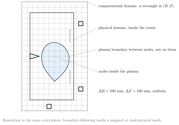
vaft.diagram.structured_rz_grid()A structured $(R, Z)$ grid: rectangular computational domain, curved plasma boundary.
vaft.diagram.structured_rz_grid(*, n_r=13, n_z=21, labels=True)Show source vaft/diagram/_spatial.py, lines 362–407
def structured_rz_grid(*, n_r: int = 13, n_z: int = 21, labels: bool = True) -> Diagram:
r"""A structured $(R, Z)$ grid: rectangular computational domain, curved plasma boundary.
The ``n_r`` $\times$ ``n_z`` nodes span the dashed computational
rectangle, which contains the physical domain (vessel) and the coils. The
LCFS cuts through cells: a rectangular grid is not aligned with the
flux surfaces, so the boundary lies between nodes (filled: nodes inside
the plasma). Same toy flux as ``flux_model``.
"""
labels = _check_labels(labels)
n_r, n_z = _index(n_r, "n_r"), _index(n_z, "n_z")
if not (4 <= n_r <= 65 and 4 <= n_z <= 129):
raise ValueError(f"n_r must be 4-65 and n_z 4-129 integers, not {n_r!r}, {n_z!r}")
model = flux_model("diverted")
boundary = lcfs(model)
o = (0.0, 0.0)
r = np.linspace(_GRID_R[0], _GRID_R[-1], n_r)
z = np.linspace(_GRID_Z[0], _GRID_Z[-1], n_z)
items: List = [Polyline.of(_cm(boundary, o), "region plasma", role="plasma", closed=True)]
for x in r:
items.append(Polyline.of(_cm([(x, z[0]), (x, z[-1])], o), "mesh", role="grid"))
for y in z:
items.append(Polyline.of(_cm([(r[0], y), (r[-1], y)], o), "mesh", role="grid"))
items.append(_rect(r[0], z[0], r[-1], z[-1], o, "approx", "computational_boundary"))
items += _machine_items(o)
items.append(Polyline.of(_cm(boundary, o), "lcfs", role="lcfs", closed=True))
inside = [(x, y) for x in r for y in z if _encloses(boundary, (x, y))]
if not inside:
raise ValueError(f"a {n_r} x {n_z} grid puts no node inside the plasma; refine it")
items += [Marker(tuple(_cm(p, o)), ".", "grid node", role="plasma_node") for p in inside]
if labels:
xl = _cm((r[-1], 0), o)[0] + 0.9
items += _leader((r[-1], z[-1]), o, (xl, 4.6), "computational domain: a rectangle in $(R, Z)$",
"computational_boundary")
items += _leader((1.05, 0.3), o, (xl, 2.6), "physical domain: inside the vessel", "vessel")
items += _leader((float(boundary[:, 0].max()), 0.0), o, (xl, 0.6),
"plasma boundary between nodes, not on them", "lcfs")
items += _leader(inside[len(inside) // 2], o, (xl, -1.4), "nodes inside the plasma", "plasma_node")
items.append(Label((xl, -3.2), f"$\\Delta R = {1e3 * (r[1] - r[0]):.0f}$ mm, "
f"$\\Delta Z = {1e3 * (z[1] - z[0]):.0f}$ mm, uniform", "small label", anchor="west",
role="spacing"))
items.append(_note("Resolution is the same everywhere; boundary-following needs a mapped or "
"unstructured mesh", 6.0, -5.6))
return Diagram("structured_rz_grid", Scene(tuple(items)),
model={"n_r": n_r, "n_z": n_z, "dr": float(r[1] - r[0]), "dz": float(z[1] - z[0]),
"n_inside": len(inside)})Formats .svg .tex .pdf the SVG above is committed; build the others locally
import vaft.diagram
d = vaft.diagram.structured_rz_grid()
d.tikz # the TikZ document as text
d.save("structured_rz_grid.svg") # rendered vector image, the canonical artifact; needs latex, dvisvgm
d.save("structured_rz_grid.tex") # the complete TikZ document, the text source
d.save("structured_rz_grid.pdf") # vector PDF; needs pdflatexgeometry_to_mesh
1 asset
source
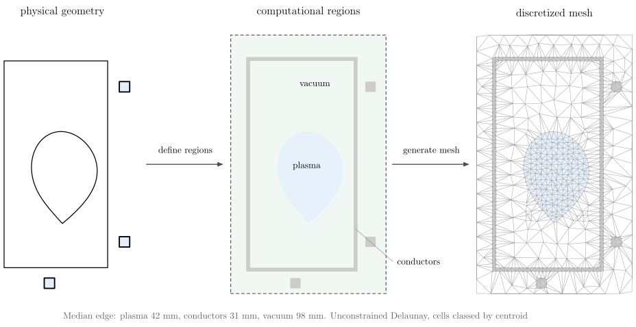
vaft.diagram.geometry_to_mesh()Geometry, then regions, then mesh: the numerical workflow, not one code’s.
vaft.diagram.geometry_to_mesh(*, labels=True)Show source vaft/diagram/_spatial.py, lines 501–564
def geometry_to_mesh(*, labels: bool = True) -> Diagram:
r"""Geometry, then regions, then mesh: the numerical workflow, not one code's.
Left, the physical geometry: wall, coils, plasma boundary. Middle, the
regions a solver distinguishes: plasma, vacuum and conductors (vessel
wall, coils). Right, an unstructured triangular mesh of the
computational box whose resolution follows the region
(:data:`MESH_SPACING`: fine in the plasma and conductors, coarse in the
vacuum) -- from :func:`unstructured_mesh`.
"""
labels = _check_labels(labels)
model = flux_model("diverted")
boundary = lcfs(model)
mesh = unstructured_mesh()
dx = 9.5
panels = [(0.0, 0.0), (dx, 0.0), (2 * dx, 0.0)]
r0, r1, z0, z1 = float(_GRID_R[0]), float(_GRID_R[-1]), float(_GRID_Z[0]), float(_GRID_Z[-1])
v0, v1, w0, w1 = _VESSEL
items: List = []
# geometry
o = panels[0]
items += [_rect(v0, w0, v1, w1, o, "machine", "vessel"),
Polyline.of(_cm(boundary, o), "lcfs", role="lcfs", closed=True)]
items += _coil_items(model["coils"], o)
# regions
o = panels[1]
items += [_rect(r0, z0, r1, z1, o, "region vacuum", "region:vacuum"),
_rect(v0 - _WALL, w0 - _WALL, v1 + _WALL, w1 + _WALL, o, "region conductor", "region:conductor"),
_rect(v0, w0, v1, w1, o, "region vacuum", "region:vacuum"),
Polyline.of(_cm(boundary, o), "region plasma", role="region:plasma", closed=True)]
items += [_rect(rc - 0.04, zc - 0.04, rc + 0.04, zc + 0.04, o, "region conductor", "region:conductor")
for rc, zc, _ in model["coils"]]
items.append(_rect(r0, z0, r1, z1, o, "approx", "computational_boundary"))
# mesh
o = panels[2]
for t, region in zip(mesh["triangles"], mesh["regions"]):
if region != "vacuum":
items.append(Polyline.of(_cm(mesh["nodes"][t], o), f"region {region}", role=f"cell:{region}",
closed=True))
nodes_cm = _cm(mesh["nodes"], o)
for i, j in mesh["edges"]:
items.append(Polyline.of([tuple(nodes_cm[i]), tuple(nodes_cm[j])], "mesh", role="edge"))
top = 5.0 * z1 + 0.6
for a, b, text in ((panels[0], panels[1], "define regions"), (panels[1], panels[2], "generate mesh")):
xa, xb = a[0] + 5.0 * r1 + 0.25, b[0] + 5.0 * r0 - 0.25
items.append(Arrow((xa, 0.0), (xb, 0.0), "connector", role="flow"))
if labels:
items.append(Label((0.5 * (xa + xb), 0.25), text, "small label", anchor="south", role="flow"))
if labels:
for o, text in zip(panels, ("physical geometry", "computational regions", "discretized mesh")):
items.append(Label((o[0] + 2.5 * (r0 + r1), top), text, "label", anchor="south", role="title"))
o = panels[1]
items += [Label(tuple(_cm(model["axis"], o)), "plasma", "small label", role="region:plasma"),
Label(tuple(_cm((0.75, 0.62), o)), "vacuum", "small label", role="region:vacuum"),
Polyline.of([tuple(_cm((v1 + _WALL / 2, -0.5), o)), tuple(_cm((r1 + 0.05, -0.75), o))],
"leader line", role="leader:conductor"),
Label(tuple(_cm((r1 + 0.06, -0.75), o)), "conductors", "small label", anchor="west",
role="region:conductor")]
m = mesh["median_edge"]
items.append(_note(f"Median edge: plasma {1e3 * m['plasma']:.0f} mm, conductors "
f"{1e3 * m['conductor']:.0f} mm, vacuum {1e3 * m['vacuum']:.0f} mm. "
"Unconstrained Delaunay, cells classed by centroid", panels[1][0] + 3.0, 5.0 * z0 - 0.6))
return Diagram("geometry_to_mesh", Scene(tuple(items)),
model={"median_edge": mesh["median_edge"], "count": mesh["count"], "spacing": dict(MESH_SPACING)})Formats .svg .tex .pdf the SVG above is committed; build the others locally
import vaft.diagram
d = vaft.diagram.geometry_to_mesh()
d.tikz # the TikZ document as text
d.save("geometry_to_mesh.svg") # rendered vector image, the canonical artifact; needs latex, dvisvgm
d.save("geometry_to_mesh.tex") # the complete TikZ document, the text source
d.save("geometry_to_mesh.pdf") # vector PDF; needs pdflatexlogical_to_physical_mapping
1 asset
source
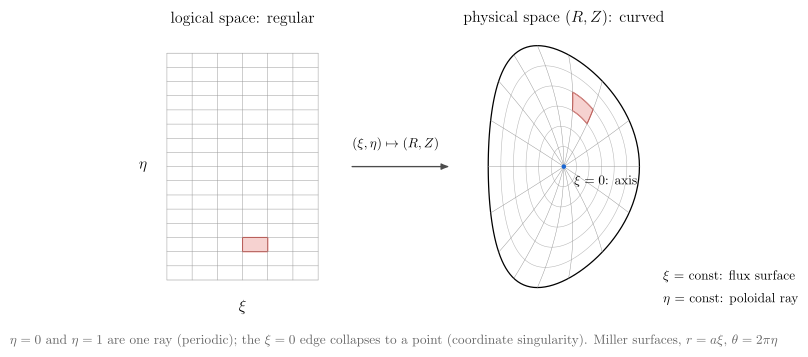
vaft.diagram.logical_to_physical_mapping()A regular logical mesh $(\xi, \eta)$ mapped onto curved flux-aligned coordinates in $(R, Z)$.
vaft.diagram.logical_to_physical_mapping(*, n_xi=6, n_eta=16, cell=(3, 2), labels=True)Show source vaft/diagram/_spatial.py, lines 578–649
def logical_to_physical_mapping(*, n_xi: int = 6, n_eta: int = 16, cell: Tuple[int, int] = (3, 2),
labels: bool = True) -> Diagram:
r"""A regular logical mesh $(\xi, \eta)$ mapped onto curved flux-aligned coordinates in $(R, Z)$.
Left, the unit square, ``n_xi`` $\times$ ``n_eta`` cells. Right, its image
under :func:`logical_to_physical`: lines of constant $\xi$ become nested
flux surfaces ($r = a\xi$ on Miller surfaces), lines of constant $\eta$
poloidal rays ($\theta = 2\pi\eta$). The shaded cell is the same cell in
both. $\eta = 0$ and $\eta = 1$ map to one ray (periodic), and $\xi = 0$
collapses to the magnetic axis -- the coordinate singularity every
flux-aligned mesh has. $\theta$ here is the mathematical angle,
counter-clockwise from the outboard midplane (as in ``tokamak_torus``),
a convention-free sketch; the sense of $\theta$ a COCOS index fixes is
what ``cocos_orientation`` draws (clockwise for COCOS 11).
"""
labels = _check_labels(labels)
n_xi, n_eta = _index(n_xi, "n_xi"), _index(n_eta, "n_eta")
if not (2 <= n_xi <= 20 and 4 <= n_eta <= 64):
raise ValueError(f"n_xi must be 2-20 and n_eta 4-64 integers, not {n_xi!r}, {n_eta!r}")
if not (isinstance(cell, tuple) and len(cell) == 2):
raise ValueError(f"cell must be an (i, j) pair, not {cell!r}")
i, j = cell
if not (0 <= i < n_xi and 0 <= j < n_eta):
raise ValueError(f"cell must index the logical mesh, not {cell!r}")
L, sx, sy = (0.0, 0.0), 4.0, 6.0 # logical square drawn 4 cm x 6 cm
phys, ps = (10.5, 0.0), 2.0 # physical panel origin and cm per m
def logical_cm(xi, eta):
return np.stack([L[0] + sx * np.asarray(xi), L[1] - 3.0 + sy * np.asarray(eta)], -1)
def physical_cm(xi, eta):
R, Z = logical_to_physical(xi, eta)
return np.stack([phys[0] + ps * (R - _MAP_SHAPE[0]), phys[1] + ps * Z], -1)
xs, es = np.linspace(0, 1, n_xi + 1), np.linspace(0, 1, n_eta + 1)
fine = np.linspace(0, 1, 121)
cxi, ceta = (xs[i], xs[i + 1]), (es[j], es[j + 1])
outline_xi = np.r_[np.linspace(*cxi, 20), np.full(20, cxi[1]), np.linspace(cxi[1], cxi[0], 20), np.full(20, cxi[0])]
outline_eta = np.r_[np.full(20, ceta[0]), np.linspace(*ceta, 20), np.full(20, ceta[1]),
np.linspace(ceta[1], ceta[0], 20)]
items: List = [Polyline.of(logical_cm(outline_xi, outline_eta), "logical cell", role="cell", closed=True),
Polyline.of(physical_cm(outline_xi, outline_eta), "logical cell", role="cell", closed=True)]
for x in xs:
items.append(Polyline.of(logical_cm(np.full(2, x), [0, 1]), "mesh", role="logical:xi"))
if x > 0:
items.append(Polyline.of(physical_cm(np.full_like(fine, x), fine),
"lcfs" if x == 1 else "surface", role="physical:xi", closed=True))
for e in es:
items.append(Polyline.of(logical_cm([0, 1], np.full(2, e)), "mesh", role="logical:eta"))
if e < 1:
items.append(Polyline.of(physical_cm(fine, np.full_like(fine, e)), "mesh", role="physical:eta"))
items.append(Marker(tuple(physical_cm(0.0, 0.0)), "o", "opoint", role="axis"))
items.append(Arrow((L[0] + sx + 0.9, 0.0), (phys[0] - ps * 1.2 - 0.6, 0.0), "connector", role="mapping"))
if labels:
items += [Label((L[0] + 0.5 * sx, -3.4), "$\\xi$", "label", anchor="north", role="logical:xi"),
Label((L[0] - 0.4, 0.0), "$\\eta$", "label", anchor="east", role="logical:eta"),
Label((L[0] + 0.5 * sx, 3.6), "logical space: regular", "label", anchor="south", role="title"),
Label((phys[0], 3.6), "physical space $(R, Z)$: curved", "label", anchor="south", role="title"),
Label((0.5 * (L[0] + sx + phys[0] - ps * 1.2), 0.3), "$(\\xi, \\eta) \\mapsto (R, Z)$",
"small label", anchor="south", role="mapping"),
Label((phys[0] + ps * 1.25, -2.9), "$\\xi$ = const: flux surface", "small label", anchor="west",
role="physical:xi"),
Label((phys[0] + ps * 1.25, -3.5), "$\\eta$ = const: poloidal ray", "small label", anchor="west",
role="physical:eta"),
Label(tuple(physical_cm(0.0, 0.0) + [0.15, -0.1]), "$\\xi = 0$: axis", "small label",
anchor="north west", role="axis"),
_note("$\\eta = 0$ and $\\eta = 1$ are one ray (periodic); the $\\xi = 0$ edge collapses to a "
"point (coordinate singularity). Miller surfaces, $r = a\\xi$, $\\theta = 2\\pi\\eta$",
6.0, -4.3)]
return Diagram("logical_to_physical_mapping", Scene(tuple(items)),
model={"shape": dict(zip(("R0", "a", "kappa", "delta"), _MAP_SHAPE)), "cell": cell,
"n_xi": n_xi, "n_eta": n_eta})Formats .svg .tex .pdf the SVG above is committed; build the others locally
import vaft.diagram
d = vaft.diagram.logical_to_physical_mapping()
d.tikz # the TikZ document as text
d.save("logical_to_physical_mapping.svg") # rendered vector image, the canonical artifact; needs latex, dvisvgm
d.save("logical_to_physical_mapping.tex") # the complete TikZ document, the text source
d.save("logical_to_physical_mapping.pdf") # vector PDF; needs pdflatexFormula functions referenced:
equilibrium.miller_surface
physical_to_flux_mapping
1 asset
source
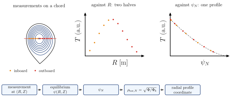
vaft.diagram.physical_to_flux_mapping()Measurements at $(R, Z)$ become a profile in $\psi_N$: two halves of a chord, one curve.
vaft.diagram.physical_to_flux_mapping(*, n_points=11, labels=True)Show source vaft/diagram/_spatial.py, lines 662–731
def physical_to_flux_mapping(*, n_points: int = 11, labels: bool = True) -> Diagram:
r"""Measurements at $(R, Z)$ become a profile in $\psi_N$: two halves of a chord, one curve.
Left, ``n_points`` measurement positions on a horizontal chord through the
magnetic axis of the toy equilibrium. Middle, a profile that depends on
$\psi_N$ only, against $R$: in- and outboard halves differ (the axis is
shifted). Right, the same values against
$\psi_N = (\psi_\mathrm{axis} - \psi)/(\psi_\mathrm{axis} - \psi_b)$ from
the equilibrium: the halves fall on one curve. $\rho_{\mathrm{tor},N} =
\sqrt{\Phi/\Phi_b}$ relabels $\psi_N$ again, through $q(\psi)$.
"""
labels = _check_labels(labels)
n_points = _index(n_points, "n_points")
if not 4 <= n_points <= 40:
raise ValueError(f"n_points must be an integer from 4 to 40, not {n_points!r}")
from scipy.interpolate import RectBivariateSpline
model = flux_model("diverted")
boundary = lcfs(model)
spline = RectBivariateSpline(_GRID_R, _GRID_Z, model["psi"])
z_chord = model["axis"][1]
on_chord = boundary[np.argsort(np.abs(boundary[:, 1] - z_chord))[:40]]
r_in = float(on_chord[on_chord[:, 0] < model["axis"][0], 0].max())
r_out = float(on_chord[on_chord[:, 0] > model["axis"][0], 0].min())
R = np.linspace(r_in, r_out, n_points + 2)[1:-1]
psi = spline(R, np.full_like(R, z_chord), grid=False)
psi_n = (model["psi_axis"] - psi) / (model["psi_axis"] - model["psi_boundary"])
value = _profile(psi_n)
inboard = R < model["axis"][0]
o = (0.0, 0.0)
items: List = _surfaces(model, o, inside_only=True)
items += [Polyline.of(_cm(boundary, o), "lcfs", role="lcfs", closed=True),
Marker(tuple(_cm(model["axis"], o)), "o", "opoint", role="axis"),
Polyline.of(_cm([(r_in - 0.05, z_chord), (r_out + 0.05, z_chord)], o), "diagnostic chord",
role="chord")]
items += [Marker(tuple(_cm((r, z_chord), o)), "o", "diagnostic inboard" if inner else "diagnostic point",
role="measurement") for r, inner in zip(R, inboard)]
charts = []
for k, (x, x_range, x_label) in enumerate(((R, (r_in, r_out), "$R$ [m]"), (psi_n, (0.0, 1.0), "$\\psi_N$"))):
chart = Chart(x_range=x_range, y_range=(0.0, 1.1))
offset, scale = (7.5 + 7.5 * k, -1.6), 0.55
if k == 1:
chart.curves["profile"] = np.stack([np.linspace(0, 1, 60), _profile(np.linspace(0, 1, 60))], -1)
scene = render_chart(chart, x_label=x_label, y_label="$T$ (a.u.)",
curve_styles={"profile": "approx"} if k == 1 else {}, region_text={})
items += list(scene.transformed(scale=scale, offset=offset).items)
for xv, yv, inner in zip(x, value, inboard):
p = chart.to_cm(np.array([xv, yv]))
items.append(Marker((float(scale * p[0] + offset[0]), float(scale * p[1] + offset[1])), "o",
"diagnostic inboard" if inner else "diagnostic point", role=f"chart{k}:measurement"))
charts.append(offset)
flow = ["measurement at $(R, Z)$", "equilibrium $\\psi(R, Z)$", "$\\psi_N$",
"$\\rho_{\\mathrm{tor},N} = \\sqrt{\\Phi/\\Phi_b}$", "radial profile coordinate"]
boxes = [box(1.7 + 3.6 * n, -4.6, 3.1, 0.9, text, role=f"flow:{n}", latex=True) for n, text in enumerate(flow)]
for b in boxes:
items += list(b.items)
items += [connector(a, b, role="flow") for a, b in zip(boxes, boxes[1:])]
if labels:
items += [Label((5.0 * model["axis"][0], 2.6), "measurements on a chord", "label",
anchor="south", role="title"),
Label((charts[0][0] + 2.5, 2.6), "against $R$: two halves", "label", anchor="south",
role="title"),
Label((charts[1][0] + 2.5, 2.6), "against $\\psi_N$: one profile", "label", anchor="south",
role="title"),
Marker((0.9, -2.9), "o", "diagnostic inboard", role="legend:inboard"),
Label((1.1, -2.9), "inboard", "small label", anchor="west", role="legend:inboard"),
Marker((3.1, -2.9), "o", "diagnostic point", role="legend:outboard"),
Label((3.3, -2.9), "outboard", "small label", anchor="west", role="legend:outboard")]
return Diagram("physical_to_flux_mapping", Scene(tuple(items)),
model={"R": R, "psi_n": psi_n, "value": value, "inboard": inboard, "z_chord": z_chord})Formats .svg .tex .pdf the SVG above is committed; build the others locally
import vaft.diagram
d = vaft.diagram.physical_to_flux_mapping()
d.tikz # the TikZ document as text
d.save("physical_to_flux_mapping.svg") # rendered vector image, the canonical artifact; needs latex, dvisvgm
d.save("physical_to_flux_mapping.tex") # the complete TikZ document, the text source
d.save("physical_to_flux_mapping.pdf") # vector PDF; needs pdflatex