Ballooning formulations
Three high-$n$ ideal-ballooning formulations are available to VAFT:
- the reduced Connor–Hastie–Taylor (CHT) $s$–$\alpha$ model in
vaft.formula.stability; - Fortran DCON’s local criterion $C_A$, which VAFT reads as
ca1; - GPEC.jl’s BALOO-style ballooning $\Delta’$ and its $\alpha_{crit}$ scans (#1098).
They share a physical limit. That does not make them the same equation, the same normalisation, the same stability index or the same algorithm. This page records which of those claims hold, from the sources. It is the theory and source part (P0) of #1637. The numerical comparisons (P1–P3) need DCON and GPEC.jl runs and belong to the stability workflow.
Sources:
- VAFT
develop; - Princeton GPEC
e68d7ac2:dcon/bal.f,dcon/mercier.f,docs/tex/dcon/notebook/bal.tex; - GPEC.jl
OpenFUSIONToolkit/GPEC@0e68a055:src/LocalStability/Ballooning.jl,docs/src/ballooning.md.
Statements marked derived here are this page’s algebra, not the sources’.
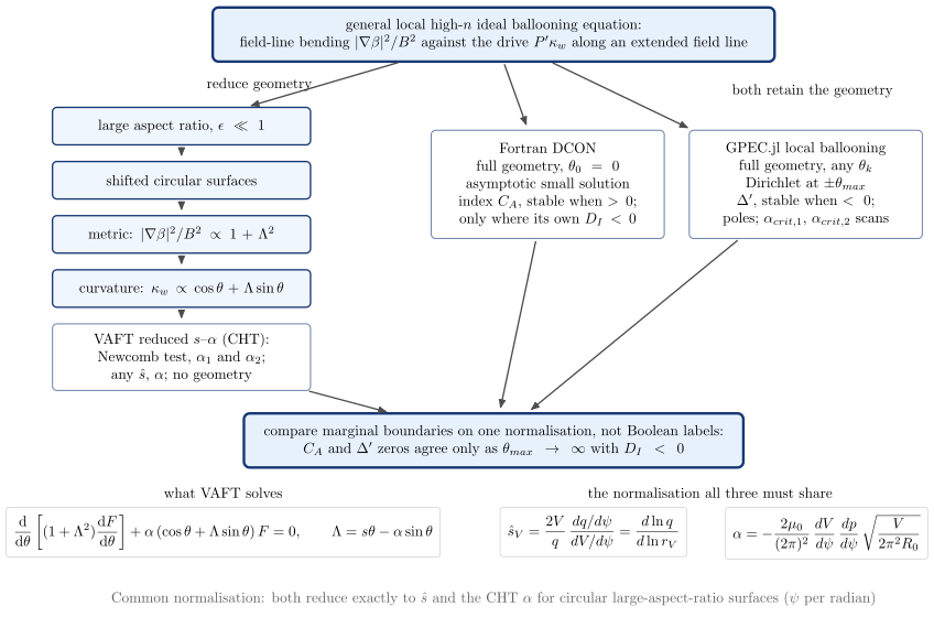
The common equation
Both full-geometry codes start from the local ballooning equation along an extended field line
\[\mathbf B\cdot\nabla\left(\frac{|\nabla\beta|^2}{B^2}\,\mathbf B\cdot\nabla\hat\varphi\right) + 2\frac{P'}{\chi'}\,\kappa_w\,\hat\varphi = 0,\qquad \kappa_w = \kappa_n - q'\theta\,\kappa_s,\]with the following conventions:
- $\beta = \zeta - q\theta + \int q’\theta_0\,d\psi$ is the field-line label;
- $P = \mu_0 p$, and primes are $d/d\psi_N$;
- $\chi’ = 2\pi\,\psi_o$, where $\psi_o$ is the poloidal flux per radian, made positive on reading;
- $\theta$ and $\zeta$ have period one (turns), not $2\pi$.
The first-order system both codes integrate is $y_1 = \hat\varphi$, $y_2 = Dy_1’$, with $y_1’ = y_2/D$ and $y_2’ = -Ky_1$. $D$ holds the field-line bending $|\nabla\beta|^2/B^2$ and $K$ holds the pressure–curvature drive.
| Field-line bending $D$ | Curvature in $K$ | Ballooning angle | |||||||
|---|---|---|---|---|---|---|---|---|---|
DCON (bal.f) |
$D = b_1(\theta - \theta_0 + b_2)^2 + b_3$, the square completed on $ | \nabla\beta | ^2/B^2$ | $\kappa_n$ from the Grad–Shafranov identity, with a $P’/B^2$ term | $\theta_0 = 0$, fixed, not an input | ||||
GPEC.jl (Ballooning.jl) |
$ | \nabla\beta | ^2/B^2 = 1/(\chi’^2 | \nabla\psi | ^2) + ( | \nabla\psi | ^2/B^2)I_{tot}^2$, with $I_{tot} = q’(\theta - \theta_k) + I_{per}$ | geometric $\kappa_n$, no GS identity, FFT-filtered derivatives | theta_k keyword, in turns |
VAFT (s_alpha_ballooning_stable) |
$1 + \Lambda^2$, $\Lambda = \hat s\theta - \alpha\sin\theta$ | $\cos\theta + \Lambda\sin\theta$ | $\theta_0 = 0$ in the solvers; $\theta$ in radians |
GPEC.jl shifts the periodic shear $I_{per}$ so that $I_{tot}(\theta_k) = 0$, and DCON does not. Their “$\theta_0 = 0$” field lines therefore coincide only for up–down symmetric equilibria.
From the general equation to $s$–$\alpha$
None of the three sources writes this reduction out. It is standard theory (CHT 1978/79; Wesson, §6.13):
- Large aspect ratio, $\epsilon \ll 1$: keep $O(1)$ in the metric and $O(\epsilon)$ in the curvature.
- Shifted circular surfaces. The Shafranov-shift gradient makes $\nabla\theta\cdot\nabla\psi \propto \sin\theta$.
- Metric. $|\nabla\zeta - q\nabla\theta|^2 \simeq (q/2\pi r)^2$ and the secular shear term $\propto \hat s\theta$. The shift adds the periodic $-\alpha\sin\theta$, so $|\nabla\beta|^2/B^2 \propto 1 + \Lambda^2$.
- Curvature. $\kappa_n \simeq -\cos\theta/R$ and $\kappa_s \propto \sin\theta/R$, so $\kappa_w \propto -(\cos\theta + \Lambda\sin\theta)$.
- Normalisation. With $\theta$ now in radians (steps 3 and 4 use the sources’ turns), $\mathbf B\cdot\nabla = (qR)^{-1}\partial_\theta$ and the drive $2P’/\chi’$ becomes $\alpha$.
This gives the CHT equation VAFT solves:
\[\frac{d}{d\theta}\left[(1 + \Lambda^2)\frac{dF}{d\theta}\right] + \alpha(\cos\theta + \Lambda\sin\theta)F = 0.\]What is lost:
- $O(\epsilon)$ metric and curvature terms;
- the poloidal variation of $B$;
- elongation and triangularity;
- the finite-$\epsilon$ harmonics of the shift.
The $s$–$\alpha$ model also lets $\alpha$ change the local shear ($-\alpha\sin\theta$) as it is scanned. DCON freezes the equilibrium’s local shear. GPEC.jl freezes it too, except for the thin-layer correction $I_{per}^{[1]}$ in its $p’$ scans.
The normalisation contract
Comparable boundaries need comparable axes. VAFT now defines both from the equilibrium’s volume, without choosing a minor radius or a field strength:
| Quantity | VAFT formula | Equation | Circular large-$\epsilon^{-1}$ limit |
|---|---|---|---|
| shear | shear_from_volume |
$\hat s_V = (2V/q)(q_\psi/V_\psi) = d\ln q/d\ln r_V$, $r_V = \sqrt{V/2\pi^2R_0}$ | exactly $\hat s = (r/q)\,dq/dr$, for any flux label |
| pressure gradient | ballooning_alpha_from_volume |
$\alpha = -(2\mu_0/(2\pi)^2)\,V_\psi\,p_\psi\,\sqrt{V/2\pi^2R_0}$ | exactly $-2\mu_0R_0q^2p’(r)/B_0^2$, with $\psi$ per radian and $R_0$ the magnetic axis |
Both identities are checked analytically in test/test_formula_ballooning_normalisation.py. With the full
flux in Wb, $\alpha$ comes out $(2\pi)^2$ too small. The older ballooning_alpha_from_p_B_R differentiates
against the major radius $R$, so it agrees only on the outboard midplane of a large-aspect-ratio circle.
GPEC.jl’s reference values are salpha_reference:
- $s_{ref} = 2Vq_\psi/(qV_\psi)$ is $\hat s_V$.
- $\alpha_{ref} = -2\mu_0\,p_\psi V_\psi\sqrt{V/2\pi R_0}$, with $\psi$ per radian, differs from the volume $\alpha$ above. Derived here: in the circular limit $\alpha_{ref} = 4\pi^{5/2}\,\alpha_{CHT} \approx 70\,\alpha_{CHT}$.
That factor must be checked numerically on an analytic large-aspect-ratio equilibrium before it is read as an inconsistency (P1). It does not affect GPEC.jl’s own scans: $\alpha_{crit} = \alpha_{ref}\times$scale, so the ratio $\alpha/\alpha_{crit}$ is invariant. It does affect any plot of absolute $\alpha$ against a CHT diagram.
Stability indices
| VAFT $s$–$\alpha$ | DCON $C_A$ | GPEC.jl ballooning $\Delta’$ | |
|---|---|---|---|
| Start / boundary | even solution $F(0) = 1$, $F’(0) = 0$ | asymptotic small solution at $-\theta_{max}$, with a first-order correction | Dirichlet $y_1 = 0$ at both $\pm\theta_{max}$ |
| Matching | none: Newcomb zero-crossing test | projection on the large / small basis at $+\theta_{max}$ | log-derivative jump at $\pm 10^{-3}$ |
| Index | Boolean; $\alpha_1$, $\alpha_2$ by bisection | $C_A$ (ca1; ca2 is not written to netCDF) |
$\Delta’ = (y_2/y_1)_R - (y_2/y_1)_L$ |
| Stable when | no zero crossing | $C_A > 0$ (derived here: the start is the small solution with $y_1 > 0$, so without a zero crossing the large-solution coefficient is positive) | $\Delta’ < 0$ (derived here, from the $P’ = 0$ limit) |
| Domain | $[0, 40\pi]$ rad, RK4, $h = 0.02$ | $\pm\min(10\,\theta_{max,0}\,\text{scale}, 100)$ turns, LSODE $10^{-5}$ | $\pm\min(10\,\text{scale}, 16.5)$ turns, DP5 $10^{-8}$ |
| Gate | none | only where $-10^4 \le D_I \le 0$ and $\psi_N \le 1$, with bal.f’s own determinant $D_I = \det\bar d_0$, not the di that mercier_scan writes to netCDF (DCON’s alpha there is the Mercier exponent $\sqrt{-D_I}$) |
none |
| Scans | $\hat s$, $\alpha$ free parameters | none | thin-layer $p’$ and $q’$ perturbations: $\alpha_{crit,1}$, $\alpha_{crit,2}$ |
How $C_A$ and $\Delta’$ relate
This section is derived here; no source states it. The Wronskian is conserved, so $\Delta’ \simeq -y_{L,1}(+\theta_{max})/[y_{L,1}(0)\,y_{R,1}(0)]$, and $C_A \simeq y_1(\theta_{max})/u_{large}$.
- The numerators play the same role: each is a solution launched at one end and evaluated at the other. The launches differ, though. A Dirichlet start carries a large-solution admixture of relative size $\theta_{max}^{-2\alpha_M}$. So the zeros coincide only as $\theta_{max} \to \infty$ with $D_I < 0$, and they differ most near Mercier-marginal surfaces. GPEC.jl’s 16.5-turn cap is much shorter than DCON’s 100.
- $\Delta’$ has poles where $y_{L,1}(0)\,y_{R,1}(0) = 0$. There it changes sign without marginality. GPEC.jl filters these heuristically: it skips a sign change when $|\Delta’| > 3|\Delta’_{anchor}|$. $C_A$ has no poles.
- $C_A$ turns positive again after a second zero crossing while the mode is still unstable. So “$C_A < 0 \Leftrightarrow$ unstable” holds only up to the first crossing. DCON counts crossings but does not write them out.
- The stable signs are opposite. Between the anchor and the first pole, $C_A$ has the sign of $-\Delta’$. They are not proportional, and not monotonic in each other.
- A single $C_A$ at the experimental equilibrium cannot give $\alpha_{crit,1}$ or $\alpha_{crit,2}$. Those need a scan.
What is left for the numerical study
These steps need solver runs; P1 must come before P2.
- P1: on an analytic large-aspect-ratio circular equilibrium, show that VAFT $s$–$\alpha$, DCON and GPEC.jl give the same first boundary after normalisation. Settle the $\alpha_{ref}$ factor first.
- P2: finite-$\epsilon$, elongation and triangularity scans.
- P3: a conventional reference equilibrium and a VEST equilibrium.
Separate convergence in $\theta_{max}$, step size and tolerance from model error. GPEC.jl’s
salpha_reference integrates $V$ from the innermost surface psilow, not from the axis. That biases $V$,
$s_{ref}$ and $\alpha_{ref}$ low near the axis, so it must be accounted for in P1 together with the
$4\pi^{5/2}$ factor. Open source questions:
- whether the $\theta_k \ne 0$ gauge difference shifts zeros on up–down asymmetric equilibria;
- how much the GS-identity and geometric $\kappa_n$ differ on equilibria that do not satisfy GS exactly;
- a bound on the Dirichlet error.
See Reduced stability diagnostics and MHD stability.
References
- J. W. Connor, R. J. Hastie and J. B. Taylor, Phys. Rev. Lett. 40 (1978) 396; Proc. R. Soc. A 365 (1979) 1.
- R. L. Miller, M. S. Chu, J. M. Greene, Y. R. Lin-Liu and R. E. Waltz, Phys. Plasmas 5 (1998) 973.
- A. H. Glasser, Phys. Plasmas 23 (2016) 072505 (DCON).
- J. Wesson, Tokamaks, 4th ed., Oxford University Press (2011), §6.13.