Plot reference
Generated from vaft.plot.registry by python -m vaft.plot.docs_catalog:
186 registered plots over 45 subjects,
plus 26 other plotting functions.
Each entry is a record of vaft.plot.available_plots(); nothing on this page is written by hand.
A plot’s identity is subject / view / quantity: the subject is what it shows physically, the view
is the kind of figure (time, profile, field, …), and the quantity picks one of several when a
subject has more than one. From data, draw a plot with its vaft.omas.plot_<name> adapter; the
renderer vaft.plot.<name> takes the typed view model instead. How the shared keywords behave is
explained on Experimental interpretation
and in the vaft.plot API.
What a plot is for is written once, in its renderer’s docstring, and read here through
vaft.plot.documentation(name): Interpretation says what the figure shows and which questions
it answers, Options what the choices that change the representation mean, and Limitations
what not to conclude from it alone. A GUI help panel reads the same parsed text. The option
values themselves are listed by vaft.omas.available_plots(ods), not repeated in the prose.
Plots not yet written to this contract show only their one-line description.
Each picture is drawn from one of the packaged sample shots by the plot’s own adapter, with
python -m vaft.plot.docs_thumbnails, and committed; the caption names the shot. A plot no packaged
sample can draw shows why instead, and a picture drawn before its renderer or sample last changed is
marked stale until it is re-rendered.
import vaft

ods = vaft.omas.sample_ods()
print(vaft.omas.available_plots(ods))              # what this input can draw
vaft.omas.plot_plasma_current_time(ods, yunit="kA")
One plot, three presentations
A plot that has a slice control (time_slice, a camera’s frame_index, the PF programme’s
time_index) can be presented three ways. They share every plot keyword; only the choice of state
differs: one index, a slider over all of them, or a sequence. Camera frames are packaged with
shot 40600:
ods = vaft.omas.sample_ods(40600)
vaft.omas.plot_camera_visible_image(ods, frame_index=120)                    # one state: a figure
vaft.omas.plot_camera_visible_image(ods, interactive=True)                   # a slider over the states
movie = vaft.omas.plot_camera_visible_image(ods, time_range=(0.3095, 0.3105), animation=True, fps=10)
movie.save("camera.mp4")                                                     # or .webm, .gif
animation=True animates the same slice control the slider moves. It draws exactly the selected
states, one frame each, with no interpolation. The whole sequence uses one colour scale.
The scientific coordinate is not the playback time:
fps=orduration=sets only how fast the frames are shown.- Each frame’s physical time is written to
movie.metadataand to thecamera.mp4.jsonsidecar.
Moving through a sequence
Every plot with more than one state to show describes how to move through them in one record,
vaft.omas.available_plots(ods).find(name).sequence. Its shape is the same for all three
kinds of storage:
kind |
option (picks one state) |
Example | States |
|---|---|---|---|
samples |
time_index |
PF programme of vacuum_field; shared magnetics grid of *_spatial_* |
every sample index |
frames |
frame_index |
the stored frames of camera_visible_image* |
every frame index |
stored |
time_slice |
the stored equilibrium reconstructions of a profile or 2-D map | the usable slices only |
The record holds the following:
states: the valuesoptionaccepts.selected: the state the static call draws, which is where a slider starts.coordinate/unit/start/stop: what the states mean.
The storage keywords keep their meaning, and navigation is the same for all of them:
- One selector at a time.
time=picks an instant: it snaps to the nearest stored frame, sample or slice. The exception isvacuum_field, which computes the field at that instant from the PF programme. Combiningtime=with an index keyword is refused instead of one silently winning. - One state set for everyone. The
interactive=Trueslider andanimation=Trueboth move through exactlystates. - Labels are times, not indices. Each state’s physical value comes from the data, never from the index alone, so a frame or slider label is the time that state was recorded.
- Usability is not validity. A state that exists but whose data are flagged remains in the
sequence, and
validity=decides how its flags are drawn. Only a state that cannot be drawn at all, such as an unusable equilibrium slice, is left out.
The output suffix picks the writer, and no backend name appears in the call:
.mp4/.webmneed the optionalvaft[video]extra (PyAV)..gifneeds nothing beyond Matplotlib.
Several plots in one figure
A vaft.plot.FigureComposition places several canonical plots in one figure: a grid of cells, each
naming a plot, its keywords and the region it covers (rowspan/colspan), and the axes that move
together. vaft.omas.compose (or vaft.imas.compose) draws it from data:
from vaft.plot import FigureCell, FigureComposition

ods = vaft.omas.sample_ods()

# m x 1: stacked time traces on one time axis, tick labels on the bottom one only
stack = FigureComposition.stack(
    ["plasma_current_time", "flux_loop_time_voltage", "equilibrium_time_q95"], panel_labels=True,
)
figure, axes = vaft.omas.compose(stack, ods)

# a map over two rows beside two profiles
equilibrium = FigureComposition(
    shape=(2, 2),
    cells=(
        FigureCell("equilibrium_field_psi", row=0, col=0, rowspan=2),
        FigureCell("equilibrium_profile_pressure", row=0, col=1),
        FigureCell("equilibrium_profile_q", row=1, col=1, options={"coordinate": "psi_norm"}),
    ),
)
figure, axes = vaft.omas.compose(equilibrium, ods, format="double_column")
Each cell is built by the plot’s own recipe, so it shows what plot_<name> would. The keywords:
share_xlinks the x axes of the cells in each column.share_ylinks the y axes of the cells in each row.AxisLink("x", (...cell names...))links any other group.title=Nonenames the shot.panel_labels=Truemarks the cells (a), (b), …- Matplotlib returns
(Figure, axes), one axes per cell, and takesformat=/theme=/figsize=. backend="plotly"returns one Plotly figure with the same cells and links.
composition.to_dict() is plain JSON and draws the same figure again.
This is not a plot’s own layout=. That keyword spreads the series of one plot over several axes;
a composition places several plots. A cell therefore holds one panel, and an overview or a
layout="subplots" plot is refused there.
Figure options and reproducible requests
On top of a format and theme, figure_options= sets what a figure asks for explicitly. It works
on any plot and on compose, with either backend. The settings it covers:
- Axes: title, axis labels, limits and scales.
- Legend: shown or hidden, location, columns, frame.
- Ticks and grid: grid, minor ticks, tick direction.
- Type: font sizes and faces. Sizes scale with the format’s proportions.
- Series: line and marker scale.
- Scalar fields: colour map, colour range, colorbar label.
Every option left out is inherited from the format, theme or plot:
from vaft.plot import DataSource, FigureOptions, PlotRequest

ods = vaft.omas.sample_ods()
vaft.omas.plot_plasma_current_time(
    ods, format="single_column", theme="technical",
    figure_options={"xlim": (0.30, 0.33), "legend": False, "minor_ticks": True},
)

request = PlotRequest(
    DataSource("sample", (39915,)), plot="plasma_current_time",
    format="single_column", figure_options=FigureOptions(xlim=(0.30, 0.33)),
)
figure, axes = request.render()
print(request.to_python())   # the plot call that draws it
print(request.to_cli())      # vaft plot plasma_current_time --sample 39915 --format ...
A PlotRequest describes a whole figure:
- Data: samples, files or database shots.
- Content: one plot with its keywords, or a composition.
- Presentation: the format, theme, backend and options.
to_python(), to_cli() and to_dict() write only what was set, so a figure reproduced later
follows any improvement to the canonical defaults. to_python(pylustrator=True) starts
Pylustrator first, for one-off finishing by hand.
Each theme pairs its text face with a MathText font. Vector files written by save_figure keep
their text as text: TrueType embedded in PDF, <text> in SVG.
Index
| Plot | View | Quantity | Description |
|---|---|---|---|
| plasma_current [ip, I_p] | |||
plasma_current_time | time | Measured plasma current history from the Rogowski coil. | |
| diamagnetic_flux | |||
diamagnetic_flux_time | time | Measured diamagnetic flux history. | |
| electron_density [ne, n_e] | |||
electron_density_time | time | Volume-averaged electron density history. | |
electron_density_profile | profile | Core electron density profile. | |
electron_density_profile_gradient | profile | gradient | Normalized logarithmic gradient of the core electron density, -L d ln f/dx, with its abscissa, gradient coordinate and reference length stated (a/L by default). |
electron_density_field | field | Electron density mapped onto the poloidal plane. | |
| electron_temperature [te, T_e] | |||
electron_temperature_time | time | Volume-averaged electron temperature history. | |
electron_temperature_profile | profile | Core electron temperature profile. | |
electron_temperature_profile_gradient | profile | gradient | Normalized logarithmic gradient of the core electron temperature, -L d ln f/dx, with its abscissa, gradient coordinate and reference length stated (a/L by default). |
electron_temperature_field | field | Electron temperature mapped onto the poloidal plane. | |
| ion_temperature [ti, T_i] | |||
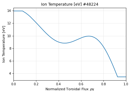
ion_temperature_profile | profile | Core ion temperature profile. | |
ion_temperature_profile_gradient | profile | gradient | Normalized logarithmic gradient of the core ion temperature, -L d ln f/dx, with its abscissa, gradient coordinate and reference length stated (a/L by default). |
| thermal_pressure [kinetic_pressure] | |||
thermal_pressure_profile | profile | Core total pressure profile. | |
| limiter_current [limiter_shunt] | |||
limiter_current_time | time | Lower-corner, upper-corner and midplane limiter currents in three panels. | |
| flux_loop | |||
flux_loop_time_flux | time | flux | Poloidal flux measured by each selected flux loop. |
flux_loop_time_voltage | time | voltage | Loop voltage measured by each selected flux loop. |
flux_loop_spatial_flux | spatial | flux | Flux-loop flux against sensor position at one time: height (inboard and outboard panels) or poloidal angle about the layout centre. |
| b_field_probe [b_pol_probe, bpol_probe] | |||
b_field_probe_time_field | time | field | Poloidal field measured by each selected B-field probe. |
b_field_probe_spatial_field | spatial | field | B-probe field against sensor position at one time: height (inboard and outboard panels) or poloidal angle about the layout centre. |
| mirnov [mirnov_coil] | |||
mirnov_time_voltage | time | voltage | Raw or preprocessed Mirnov coil voltage traces. |
mirnov_spatial_phase | spatial | phase | Toroidal phase of each fluctuation band around the torus at one time, with the fitted n mode lines. |
mirnov_spectrum | spectrum | Power spectral density of one Mirnov coil signal. | |
mirnov_spectrogram | spectrogram | Time-frequency map of one Mirnov coil signal. | |
| impa [hall_probe_array] | |||
impa_time_field | time | field | Calibrated field from the IMPA Hall-probe array. |
impa_time_voltage | time | voltage | Raw IMPA Hall-probe voltages, one trace per channel. |
impa_profile_field | profile | field | IMPA measured field against probe radius with the 1/R toroidal-field model. |
impa_overview | overview | IMPA validation overview: raw voltages, compensated Bz and the 1/R position check. | |
| soft_x_rays [soft_x_ray, sxr] | |||
soft_x_rays_time_power | time | power | Soft X-ray channel signal history. |
soft_x_rays_geometry_lines_of_sight | geometry | lines_of_sight | Soft X-ray detector lines of sight over the poloidal cross-section. |
soft_x_rays_spectrum | spectrum | Power spectral density of one soft X-ray channel. | |
soft_x_rays_spectrogram | spectrogram | Time-frequency map of one soft X-ray channel. | |
soft_x_rays_overview | overview | channels | Soft X-ray overview: lines of sight, signals and channel pattern. |
| interferometer | |||
interferometer_time_n_e_line | time | n_e_line | Interferometer line-integrated electron density history. |
interferometer_spectrum | spectrum | Power spectral density of one interferometer channel's line density. | |
interferometer_spectrogram | spectrogram | Time-frequency map of one interferometer channel's line density. | |
interferometer_overview | overview | channels | Interferometer overview: line density history and spectrogram. |
| thomson_scattering [thomson] | |||
thomson_scattering_time_electron_density | time | electron_density | Per-channel Thomson electron density history. |
thomson_scattering_time_electron_temperature | time | electron_temperature | Per-channel Thomson electron temperature history. |
thomson_scattering_profile_electron_density | profile | electron_density | Thomson-scattering electron density versus position. |
thomson_scattering_profile_electron_temperature | profile | electron_temperature | Thomson-scattering electron temperature versus position. |
thomson_scattering_profile_fit | profile | fit | Thomson T_e or n_e (field=te|ne) at one time: channels with error bars, refused channels hollow, and the fit through them on psi_N, rho_N or R, mapped through the ODS's own or a given equilibrium (issue #952). |
thomson_scattering_geometry_poloidal | geometry | poloidal | Thomson-scattering measurement positions in the poloidal plane. |
| charge_exchange | |||
charge_exchange_time_ion_temperature | time | ion_temperature | Per-channel ion temperature history from charge-exchange spectroscopy. |
charge_exchange_time_velocity_tor | time | velocity_tor | Per-channel toroidal rotation history from charge-exchange spectroscopy. |
charge_exchange_profile_fit | profile | fit | Charge-exchange T_i or V_phi (field=ti|vphi) at one time: channels with error bars, refused channels hollow, and the fit through them on psi_N, rho_N or R (issue #952). |
charge_exchange_profile_ion_temperature | profile | ion_temperature | Charge-exchange ion temperature versus position. |
charge_exchange_profile_velocity_tor | profile | velocity_tor | Charge-exchange toroidal rotation versus position. |
charge_exchange_geometry_poloidal | geometry | poloidal | Charge-exchange measurement positions in the poloidal plane. |
| spectrometer_uv | |||
spectrometer_uv_time_impurity | time | impurity | Impurity line-intensity panels against plasma current. |
spectrometer_uv_time_intensity | time | intensity | Processed spectral line intensity history. |
| barometry | |||
barometry_time_pressure | time | pressure | Neutral pressure history from the barometry gauges. |
| rogowski_coil [rogowski] | |||
rogowski_coil_time_current | time | current | Current measured by each Rogowski coil. |
| camera_visible | |||
camera_visible_spectrogram | spectrogram | Time-frequency map of the FAST-camera intensity summed over one image region, the camera side of the published camera/magnetics comparison (issue #161). | |
camera_visible_image | image | One camera frame with optional overlays -- wall, equilibrium, field line -- through one projection (issue #261). | |
camera_visible_image_efit_overlay | image | efit_overlay | FAST-camera frame with the calibrated pinhole projection of the wall, LCFS, magnetic axis, and flux surfaces overlaid. |
camera_visible_image_field_line | image | field_line | FAST-camera frame with a traced magnetic field line projected onto it. |
camera_visible_image_fluctuation | image | fluctuation | One FAST-camera frame with its local temporal background removed, the published step that brings fast filamentary structure out of the slowly varying line emission (issue #161). |
camera_visible_image_frame | image | frame | One FAST-camera frame (raw digital levels, uncalibrated). |
camera_visible_image_mhd_power | image | mhd_power | Per-pixel MHD-band power divided by the local average emission: the published spectrally filtered image, which is a band magnitude and not an inverse-transform reconstruction (issue #161). |
camera_visible_image_vacuum_field_line | image | vacuum_field_line | FAST-camera frame with vacuum field lines -- coils and vessel only, never an equilibrium -- traced from (R, Z) seeds at the frame's time (seeds=, ec_frequency_Hz= adds the ECR radius). |
camera_visible_animation_frames | animation | frames | Animate a sequence of FAST-camera frames on a shared color scale. |
| magnetics | |||
magnetics_geometry_poloidal | geometry | poloidal | Flux-loop and B-field-probe positions in the poloidal plane. |
magnetics_overview | overview | diagnostics | Shot diagnostic overview: current, field, flux and geometry panels. |
magnetics_overview_plasma_residual | overview | plasma_residual | Residual of measured minus coil+eddy synthetic magnetics against the pre-plasma noise band, with the plasma-current and residual onsets. |
magnetics_overview_vacuum | overview | vacuum | Measured, coil-only and coil+eddy synthetic magnetics per channel: the forward-modeled validation of an eddy-current reconstruction. |
magnetics_overview_vacuum_benchmark | overview | vacuum_benchmark | Per-channel scores of the plasma-free vacuum benchmark (issue #190): eddy improvement against a zero reference, normalized residual and correlation, channels grouped and coloured by family, flagged probes hollow. |
magnetics_table_vacuum_benchmark | table | vacuum_benchmark | The plasma-free vacuum benchmark of one shot (issue #190), one row per channel: family, kind, status (evaluated, flagged, excluded), eddy improvement, normalized residual, correlation, wall authority and the reason a channel is flagged or excluded; windows, solver history, coil drive and scored medians in the caption. |
magnetics_table_vacuum_benchmark_aggregate | table | vacuum_benchmark_aggregate | The plasma-free vacuum benchmark across shots (issue #190): median eddy improvement, normalized residual and correlation and the worst channel by case, family, PF excitation and machine era; undriven cases, flagged channels and the summary in the caption. |
| wall | |||
wall_geometry_poloidal | geometry | poloidal | First-wall and limiter outline in the poloidal plane. |
| pf_coil [pf_active] | |||
pf_coil_time_current | time | current | Per-coil PF current history. |
pf_coil_time_current_turns | time | current_turns | Per-coil PF current multiplied by the signed turn count (ampere-turns). |
pf_coil_geometry_poloidal | geometry | poloidal | PF coil cross-sections in the poloidal plane: every element of every coil, as the rectangle or outline the IDS stores. |
| tf_coil [tf] | |||
tf_coil_time_b_t | time | b_t | Toroidal field history at the reference radius. |
tf_coil_time_b_t_vacuum_r | time | b_t_vacuum_r | Vacuum toroidal field times major radius (B_t * R). |
tf_coil_time_current | time | current | TF coil current history. |
| passive_structure [pf_passive] | |||
passive_structure_time_current | time | current | Eddy current induced in the passive structure, summed over loops. |
passive_structure_field_wall_reduction | field | wall_reduction | The passive wall's poloidal flux on the equilibrium region -- full, reduced, or their difference -- at one instant of the shot's PF programme (vaft #494, vfit #10). |
passive_structure_geometry_poloidal | geometry | poloidal | Passive conducting structure in the poloidal plane: every loop element, drawn as one structure rather than one object per loop. |
passive_structure_geometry_wall_mode | geometry | wall_mode | One eigenmode of the passive wall: every loop of the chosen segment coloured by its signed relative current, the rest grey (vaft #473; the reduced-wall contract, vfit #8). |
passive_structure_overview_wall_reduction | overview | wall_reduction | Reduced-wall response error against retained order, one panel per metric and one series per selection rule: how much of the wall's own contribution a truncated basis misses (vaft #494, vfit #10). |
passive_structure_overview_wall_time | overview | wall_time | Decay-time spectrum of the passive wall's segment-wise eigenmodes: one series per conductor segment, slowest mode first, with the whole wall's global spectrum for reference (vaft #473). |
| pf_plasma [plasma_elements, plasma_current_elements] | |||
pf_plasma_geometry_poloidal | geometry | poloidal | The plasma current as pf_plasma elements (filaments or a grid of current elements), each coloured by its signed current at one instant. |
| coil_3d [coils_non_axisymmetric, 3d_coil] | |||
coil_3d_profile_current | profile | current | Sector currents of each non-axisymmetric coil set against toroidal angle: one marker per sector, because that is the whole waveform a discrete coil set carries. |
coil_3d_geometry_topview | geometry | topview | Non-axisymmetric 3D coil filaments projected into the machine top view. |
coil_3d_geometry3d | geometry3d | Non-axisymmetric 3D coil filaments in machine Cartesian coordinates. | |
coil_3d_spectrum_current | spectrum | current | Toroidal mode content |C_n| of each non-axisymmetric coil set's excitation, to the last harmonic its sectors resolve. |
| machine | |||
machine_geometry_poloidal | geometry | poloidal | Composed poloidal machine view: wall, coils, passive structure and diagnostic positions and sight lines in one axes. |
machine_geometry_topview | geometry | topview | Composed machine top view: machine-boundary and plasma extent, launcher, antenna and pellet-injector geometry, and the toroidal position of every diagnostic channel that stores one. |
machine_geometry3d | geometry3d | Composed 3D machine scene: wall and plasma-boundary cuts at four toroidal angles, PF coil rings, non-axisymmetric coils, and every diagnostic channel that stores r, phi and z. | |
| equilibrium | |||
equilibrium_time_beta | time | beta | Poloidal, toroidal and normalized beta panels. |
equilibrium_time_beta_n | time | beta_n | Normalized beta history. |
equilibrium_time_beta_p | time | beta_p | Poloidal beta history. |
equilibrium_time_beta_t | time | beta_t | Toroidal beta history. |
equilibrium_time_diamagnetic_flux | time | diamagnetic_flux | Measured versus reconstructed diamagnetic-flux constraint. |
equilibrium_time_elongation | time | elongation | Boundary elongation history. |
equilibrium_time_li | time | li | Internal inductance li_3 history. |
equilibrium_time_major_radius | time | major_radius | Geometric-axis major radius history. |
equilibrium_time_minor_radius | time | minor_radius | Boundary minor radius history. |
equilibrium_time_plasma_current | time | plasma_current | Reconstructed plasma current history. |
equilibrium_time_q0 | time | q0 | Safety factor on axis. |
equilibrium_time_q95 | time | q95 | Safety factor at the 95% flux surface. |
equilibrium_time_qa | time | qa | Safety factor at the plasma edge. |
equilibrium_time_shape | time | shape | Major and minor radius, elongation and upper/lower triangularity histories. |
equilibrium_time_triangularity | time | triangularity | Boundary triangularity history, the mean of upper and lower. |
equilibrium_time_triangularity_lower | time | triangularity_lower | Lower boundary triangularity history. |
equilibrium_time_triangularity_upper | time | triangularity_upper | Upper boundary triangularity history. |
equilibrium_time_virial | time | virial | Virial-estimate equilibrium quantities against the reconstruction. |
equilibrium_time_w_mag | time | w_mag | Magnetic stored energy history. |
equilibrium_time_w_mhd | time | w_mhd | MHD stored energy history. |
equilibrium_time_w_tot | time | w_tot | Total stored energy history. |
equilibrium_profile_f | profile | f | Equilibrium poloidal current function F = R*B_t. |
equilibrium_profile_ffprime | profile | ffprime | Equilibrium F dF/dpsi profile. |
equilibrium_profile_j_tor | profile | j_tor | Equilibrium toroidal current-density profile. |
equilibrium_profile_pprime | profile | pprime | Equilibrium dp/dpsi profile. |
equilibrium_profile_pressure | profile | pressure | Equilibrium 1D pressure profile. |
equilibrium_profile_q | profile | q | Equilibrium safety-factor profile. |
equilibrium_field_2d | field | 2d | Any reconstructed 2-D equilibrium quantity on the (R, Z) grid: flux, current density, pressure or field, with the machine drawn over it. |
equilibrium_field_psi | field | psi | Reconstructed poloidal flux map on the equilibrium (R, Z) grid. |
equilibrium_field_psi_vacuum | field | psi_vacuum | Vacuum poloidal flux from the PF coils alone, without plasma. |
equilibrium_geometry_boundary | geometry | boundary | Last-closed-flux-surface outline in the poloidal plane. |
equilibrium_geometry_topview | geometry | topview | Equilibrium boundary projected into the machine top view. |
equilibrium_overview | overview | analysis | One equilibrium slice from one figure: poloidal flux with the LCFS and axis, pressure and q profiles, and the slice's global quantities. |
equilibrium_overview_constraint_coverage | overview | constraint_coverage | Enabled, disabled and missing constraint channels per family across the reconstructed time slices. |
equilibrium_overview_constraint_weights | overview | constraint_weights | Per constraint family: the stored uncertainty beside the one EFIT fitted against (k / weight), the weight, and the normalized residual (issue #952). |
equilibrium_overview_constraints | overview | constraints | Magnetic constraints as submitted to EFIT, per family, with enabled, disabled and missing channels distinguished. |
equilibrium_overview_convergence | overview | convergence | EFIT numerical convergence: final Grad-Shafranov error against the requested tolerance, iteration count against its cap, the error history where one was written, and EFIT's outputs checked against each other. |
equilibrium_overview_fit_quality | overview | fit_quality | EFIT goodness of fit: reduced chi-square against the degrees of freedom EFIT itself reports, which diagnostic family carries the chi-square, and residuals normalized by the uncertainty EFIT was given. |
equilibrium_overview_histories | overview | histories | Equilibrium global quantities against time: Ip, beta_p, li, q95. |
equilibrium_overview_pressure_weight_scan | overview | pressure_weight_scan | Reconstructions of one instant with the kinetic-pressure constraint weighted differently, entries labelled by the factor: p and q against psi_N, and beta_p, l_i and chi-square against the factor (issue #952). |
equilibrium_overview_profiles | overview | profiles | Principal 1-D equilibrium profiles: pressure, toroidal current density and safety factor. |
equilibrium_overview_residuals | overview | residuals | Measured-minus-reconstructed residuals by diagnostic family, with the solver's convergence context beside them rather than in place of them. |
equilibrium_overview_verification | overview | verification | EFIT verification overview: measured and reconstructed constraints beside the reconstructed poloidal-flux map. |
equilibrium_table_fit_quality | table | fit_quality | EFIT goodness of fit at one slice, per constraint family: fit role, channel states, share of the total chi-square and residuals normalized by the uncertainty EFIT was given; the reduced chi-square in the caption. |
equilibrium_table_summary | table | summary | One equilibrium slice's global quantities as a table -- the representative slice, or the stored slice time= snaps to -- in the display units of the slice overview. |
equilibrium_table_validation | table | validation | Every registered validation check's verdict at one equilibrium slice -- verification, diagnostic fit, physical validity, independent validation: the number each status was decided on, the registry criterion, the status (NOT_AVAILABLE and INDETERMINATE kept as such) and its reason; the aggregate status and the count per status in the caption. |
equilibrium_text_summary | text | summary | One equilibrium slice as a text summary: which slice and why, its global quantities, and its boundary shape. |
| vacuum [vacuum_field, null_field] | |||
vacuum_field | field | The vacuum field of the coils and vessel at one instant: the flux, the poloidal field strength, the decay index, |E_phi|, the breakdown figure of merit, or the Lloyd margin, chosen with field=. | |
vacuum_field_midplane | field | midplane | One vacuum startup quantity along the Z = 0 row of the vacuum map -- loop voltage, B_Z, the breakdown figure with its Ohmic and ECH-assisted thresholds, the Lloyd margin or the connection length -- with the ECR radius, chosen with field=. |
| startup_proxies [startup] | |||
startup_proxies_time | time | Vacuum B_Z, loop voltage and decay index at one (R, Z) point against time (rz=), from the OH-coil onset to the plasma-current peak, every entry overlaid with its breakdown onset marked (issue #888). | |
| core_profiles | |||
core_profiles_time_volume_averaged | time | volume_averaged | Volume-averaged core quantity panels on a shared time axis. |
core_profiles_profile_zeff | profile | zeff | Z_eff(rho) stored in a core_profiles slice, labelled measured, assumed, derived or inferred by its zeff_fit record; an unlabelled profile says so. |
| mhd_linear | |||
mhd_linear_time_energy_perturbed | time | energy_perturbed | DCON perturbed potential energy against time, one trace per toroidal mode number; a negative value is an ideal-MHD unstable mode. |
mhd_linear_profile_b_field_perturbed | profile | b_field_perturbed | Normal perturbed field per poloidal harmonic against normalized flux, derived from the DCON eigenfunction as i(m - nq) xi.grad(psi). |
mhd_linear_profile_chirikov | profile | chirikov | Island-overlap parameter per rational surface against normalized poloidal flux, in GPEC's own surface definition, with the K = 1 criterion drawn; derived from the mapped perturbed flux. |
mhd_linear_profile_displacement | profile | displacement | DCON displacement eigenfunction against normalized flux, one trace per poloidal harmonic; amplitudes are normalized to the peak because DCON's eigenvector normalization is arbitrary. |
mhd_linear_profile_island_width | profile | island_width | Saturated island width per rational surface against normalized poloidal flux, in psi_N as GPEC reports it, derived from the resonant flux. |
mhd_linear_profile_resonant_flux | profile | resonant_flux | Pitch-resonant flux per rational surface against normalized poloidal flux, derived from the mapped perturbed flux by the jump across each singular surface rather than read from the IDS. |
mhd_linear_field_spectrum | field | spectrum | Perturbed normal flux amplitude over the mapped (psi_N, m) grid: the radial label on the abscissa and the poloidal harmonic on the ordinate, which is why this map is not drawn to an equal aspect. |
mhd_linear_geometry_island | geometry | island | Saturated island separatrices in the poloidal plane at one toroidal angle, derived from the mapped perturbed flux and drawn on the run's own flux-surface mesh; the island phase is GPEC's arg(I_res). |
mhd_linear_spectrum_b_field_perturbed | spectrum | b_field_perturbed | Perturbed normal flux amplitude against poloidal harmonic at one flux surface; the outermost mapped surface unless psi_n names another, and the title reports the surface actually drawn. |
mhd_linear_overview_eigenfunction | overview | eigenfunction | The DCON eigenfunction of the least-stable mapped mode: displacement and normal perturbed field per poloidal harmonic. |
| ntms [tearing, delta_prime] | |||
ntms_time_delta_prime | time | delta_prime | Classical tearing index Delta-prime against time, one trace per rational surface; a positive value is a tearing-unstable surface. This is RDCON's and STRIDE's physical result, which has no slot under `toroidal_mode` and lives in `ntms`. |
| field_line_topology [connection_length, field_lines] | |||
field_line_topology_field_connection_length | field | connection_length | Total connection length of every traced field line in one poloidal plane, on the rectangular grid they were launched from. The title names the toroidal angle the plane was traced at, because the IDS entry carries no toroidal coordinate and the map means nothing without it. |
| neoclassical [bootstrap_current] | |||
neoclassical_profile_bootstrap_current | profile | bootstrap_current | Bootstrap current density from each neoclassical model on one radial axis: the Sauter and Redl formulas against whatever solver result the ODS carries. |
| gyrokinetics [gyrokinetics_local, local_gyrokinetics, linear_spectrum] | |||
gyrokinetics_profile_eigenfunction | profile | eigenfunction | phi eigenfunction of the most unstable leading mode against the poloidal angle. |
gyrokinetics_spectrum_energy_flux | spectrum | energy_flux | ky-resolved energy flux per species (quasilinear or nonlinear, as the IDS records). |
gyrokinetics_spectrum_frequency | spectrum | frequency | Linear real frequency against k_y with each IDS's recorded sign convention. |
gyrokinetics_spectrum_growth_rate | spectrum | growth_rate | Linear growth rate against k_y (GKDB normalisation), every eigenmode, entries overlaid. |
gyrokinetics_spectrum_particle_flux | spectrum | particle_flux | ky-resolved particle flux per species. |
gyrokinetics_overview | overview | One local gyrokinetic run: spectra, flux, eigenfunction and local state. | |
| turbulent_transport [anomalous_transport, turbulent_flux] | |||
turbulent_transport_profile_energy_flux | profile | energy_flux | Turbulent electron and ion energy flux against rho_tor_norm. |
turbulent_transport_profile_particle_flux | profile | particle_flux | Turbulent electron and ion particle flux against rho_tor_norm. |
turbulent_transport_overview | overview | Turbulent energy and particle flux profiles side by side. | |
| impurity [impurities] | |||
impurity_profile_charge_state_fraction | profile | charge_state_fraction | Charge-state fractions f_q(rho) of each impurity element from the slice's T_e and n_e. |
impurity_profile_composition | profile | composition | Radial Z_eff, mean charges, reduced impurity charge and dilution from the slice's T_e and n_e through atomic-data charge states, for a stated elemental composition. |
| nbi [neutral_beam, nubeam] | |||
nbi_profile_current_drive | profile | current_drive | Beam-driven parallel current density against normalized toroidal flux, <J.B>/B0. Derived from the solver's toroidal driven current and the equilibrium geometry, assuming the driven current is field-aligned on each flux surface; it is not a direct solver output. |
nbi_profile_electron_heating | profile | electron_heating | Beam power density to electrons against normalized toroidal flux, from a NUBEAM result mapped into core_sources. |
nbi_profile_ion_heating | profile | ion_heating | Beam power density to ions against normalized toroidal flux, from a NUBEAM result mapped into core_sources. |
| ec_launchers [ech, ecrh, electron_cyclotron] | |||
ec_launchers_time_power | time | power | Net launched electron-cyclotron power (forward minus reflected) per beam; noisy, so smooth= is a rolling median in seconds. |
| chease | |||
chease_overview_profile_validity | overview | profile_validity | q0/q95, q-monotonicity and pressure positivity of the refined equilibrium: a converged CHEASE solution that is not physically sound flagged at a glance. |
chease_overview_refinement_summary | overview | refinement_summary | How far CHEASE moved each profile and the boundary from the EFIT equilibrium it refined, slice by slice: profile and boundary RMS change, flux-normalization shift, and plasma-current self-consistency. |
| current | |||
current_overview | overview | Plasma, PF coil and eddy current panels on a shared time axis. | |
current_overview_reconstruction | overview | reconstruction | Measured I_p with the reconstructed I_p of every equilibrium slice by convergence, PF coil currents and eddy currents, in kA. |
| diagnostics | |||
diagnostics_spectrum_coherence | spectrum | coherence | Coherence (with its 95 % significance line) and relative phase of two fluctuation channels -- Mirnov, soft X-ray or interferometer -- compared on one time grid over their overlap (issue #1005). |
diagnostics_overview | overview | Time histories of every diagnostic subject, one panel each; a diagnostic absent from the input is left out and the grid shrinks (issue #476), and members= picks the panels by name (issue #482). Channels the source flagged invalid are excluded by default. | |
| kinetic | |||
kinetic_overview_profiles | overview | profiles | Local n_e, T_e, T_i and V_phi from compatible diagnostics and core-profile fits. |
kinetic_overview_state | overview | state | One matched kinetic state in four panels -- pressure, density, temperature and Z_eff against rho_tor_norm -- from stored core_profiles, the equilibrium of the same time and the Thomson channels mapped through it, each trace labelled by its recorded evidence role. |
| summary | |||
summary_time_energy | time | energy | Stored-energy comparison panels across available estimates. |
summary_time_estimated_q95 | time | estimated_q95 | q95 estimated from global shape, I_p and B_T (START scaling by default, from vest.yaml), the equilibrium q95 overlaid; works without an equilibrium (issue #1583). |
summary_time_normalized_current | time | normalized_current | Normalised current I_N = I_p[MA]/(a B_T) against time, from the same shape as the edge-q estimates (issue #1583). |
summary_time_power_balance | time | power_balance | Ohmic input, radiated and conducted power balance panels. |
summary_time_q_star_cylindrical | time | q_star_cylindrical | Menard's cylindrical safety factor q* = pi a^2 B_T (1 + kappa^2)/(mu0 R I_p) against time; a shape-weighted proxy, not q95 or q_a (issue #1583). |
summary_time_q_star_kink | time | q_star_kink | Freidberg's kink safety factor q* = 2 pi a^2 kappa B_T/(mu0 R I_p) against time; not q95 or q_a (issue #1583). |
summary_time_resistive_zeff | time | resistive_zeff | Resistive Z_eff history: Romero voltages, observed vs model R_p, window estimate. |
summary_time_romero_balance | time | romero_balance | Romero's voltage and volt-second balance: V_B, V_I, V_C (and V_R with a given R_p), Phi_B against the direct flux change, L_i and the closing resistance. |
summary_time_voltage_consumption | time | voltage_consumption | Loop-voltage and flux-consumption panels. |
No plot matches.
Quantity subjects
plasma_current [ip, I_p]
plasma_current_time · shot 39915 Staleplasma_current_time
time
source
plasma_current / time · domain magnetics · view model LineSeries
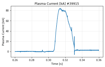
Measured plasma current history from the Rogowski coil.
Interpretation
The toroidal plasma current against time. It is the first trace read for any discharge: breakdown and current rise, flat-top, termination and current quench, and the time windows other analyses use. It normalizes many derived quantities (normalized beta, the Greenwald density, q estimates) and compares discharges at a glance.
Limitations
A Rogowski coil measures all current threading it. Depending on where it sits and on the processing that produced the stored waveform, currents induced in the vessel and passive structure may be included; they matter most at breakdown and during the current quench.
Convention · See Also
Convention
The stored sign follows the machine’s current direction in the IMAS
convention. The default display draws the dominant polarity positive and
says “sign flipped” in the title when it did; orientation="canonical"
keeps the stored sign, which is what tells the current direction.
See Also
equilibrium_time_plasma_current : the current the reconstruction fitted. current_overview : plasma, coil and eddy currents together.
Thumbnail drawn from sample shot 39915, stale: renderer or style changed.
vaft.omas.plot_plasma_current_time(ods)         # from data
vaft.plot.plasma_current_time(model)   # from a LineSeries
Show source vaft/plot/renderers/lines.py, lines 136–194
@renderer(
    domain="magnetics",
    subject="plasma_current",
    view="time",
    quantity="",
    model=LineSeries,
    description="Measured plasma current history from the Rogowski coil.",
    ids=("magnetics",),
    required_paths=(
        "magnetics.ip.0.time",
        "magnetics.ip.0.data",
    ),
    optional_paths=(),
)
def plasma_current_time(
    model: LineSeries,
    *,
    ax: Axes | None = None,
    show: bool = False,
    **style: Any,
) -> tuple[Figure, Axes]:
    """Measured plasma current history from the Rogowski coil.

    Interpretation
    --------------
    The toroidal plasma current against time.  It is the first trace read for
    any discharge: breakdown and current rise, flat-top, termination and
    current quench, and the time windows other analyses use.  It normalizes
    many derived quantities (normalized beta, the Greenwald density, q
    estimates) and compares discharges at a glance.

    Options
    -------
    ``synthetic=`` overlays, as markers at each equilibrium slice, the value
    the reconstruction predicts for this signal, so measurement and fit can be
    compared where the fit exists.  ``orientation=`` draws the current positive
    whatever the stored sign; ``x=`` replaces time by the sample index, for
    checking acquisition rather than physics.

    Convention
    ----------
    The stored sign follows the machine's current direction in the IMAS
    convention.  The default display draws the dominant polarity positive and
    says "sign flipped" in the title when it did; ``orientation="canonical"``
    keeps the stored sign, which is what tells the current direction.

    Limitations
    -----------
    A Rogowski coil measures all current threading it.  Depending on where it
    sits and on the processing that produced the stored waveform, currents
    induced in the vessel and passive structure may be included; they matter
    most at breakdown and during the current quench.

    See Also
    --------
    equilibrium_time_plasma_current : the current the reconstruction fitted.
    current_overview : plasma, coil and eddy currents together.
    """
return render_line_series(model, ax=ax, show=show, **style)| IDS | magnetics |
|---|---|
| Required paths | magnetics.ip.0.timemagnetics.ip.0.data |
| Backends | matplotlib, plotly |
| Renderer | vaft.plot.renderers.lines.plasma_current_time |
diamagnetic_flux
diamagnetic_flux_time · shot 39915 Stalediamagnetic_flux_time
time
source
diamagnetic_flux / time · domain magnetics · view model LineSeries
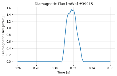
Measured diamagnetic flux history.
Interpretation
The change in toroidal flux through the plasma cross-section caused by the plasma. Through radial pressure balance it measures the perpendicular pressure relative to the poloidal field: in the large-aspect-ratio limit a plasma with poloidal beta above 1 expels toroidal flux (diamagnetic), one below it draws flux in (paramagnetic). It is the main magnetic measurement of stored energy and poloidal beta, and the one that separates beta_p from l_i in a reconstruction.
Limitations
The plasma’s contribution is small beside the vacuum toroidal flux, so the trace depends on how the toroidal-field pickup and vessel currents were compensated, and integrated signals can drift. Turning it into beta or stored energy needs the plasma shape, i.e. a reconstruction.
Convention · See Also
Convention
In VEST products a positive stored flux is a paramagnetic plasma (#1196),
a negative one a diamagnetic plasma. The sign carries that meaning only
under orientation="canonical".
See Also
equilibrium_time_beta_p : the reconstruction’s poloidal beta. equilibrium_time_diamagnetic_flux : measured against reconstructed constraint.
Thumbnail drawn from sample shot 39915, stale: renderer or style changed.
vaft.omas.plot_diamagnetic_flux_time(ods)         # from data
vaft.plot.diamagnetic_flux_time(model)   # from a LineSeries
Show source vaft/plot/renderers/lines.py, lines 197–258
@renderer(
    domain="magnetics",
    subject="diamagnetic_flux",
    view="time",
    quantity="",
    model=LineSeries,
    description="Measured diamagnetic flux history.",
    ids=("magnetics",),
    required_paths=(
        "magnetics.time",
        "magnetics.diamagnetic_flux.0.data",
    ),
    optional_paths=(),
)
def diamagnetic_flux_time(
    model: LineSeries,
    *,
    ax: Axes | None = None,
    show: bool = False,
    **style: Any,
) -> tuple[Figure, Axes]:
    """Measured diamagnetic flux history.

    Interpretation
    --------------
    The change in toroidal flux through the plasma cross-section caused by the
    plasma.  Through radial pressure balance it measures the perpendicular
    pressure relative to the poloidal field: in the large-aspect-ratio limit a
    plasma with poloidal beta above 1 expels toroidal flux (diamagnetic), one
    below it draws flux in (paramagnetic).  It is the main magnetic measurement of stored energy and
    poloidal beta, and the one that separates beta_p from l_i in a
    reconstruction.

    Options
    -------
    ``synthetic=`` overlays, as markers at each equilibrium slice, the value
    the reconstruction predicts for this signal, so measurement and fit can be
    compared where the fit exists.  By default the dominant polarity is
    drawn positive, so a diamagnetic shot, whose stored flux is negative, is
    drawn positive too and the title says "sign flipped";
    ``orientation="canonical"`` keeps the stored sign and is needed to read
    para- or diamagnetism from the plot.

    Convention
    ----------
    In VEST products a positive stored flux is a paramagnetic plasma (#1196),
    a negative one a diamagnetic plasma.  The sign carries that meaning only
    under ``orientation="canonical"``.

    Limitations
    -----------
    The plasma's contribution is small beside the vacuum toroidal flux, so the
    trace depends on how the toroidal-field pickup and vessel currents were
    compensated, and integrated signals can drift.  Turning it into beta or
    stored energy needs the plasma shape, i.e. a reconstruction.

    See Also
    --------
    equilibrium_time_beta_p : the reconstruction's poloidal beta.
    equilibrium_time_diamagnetic_flux : measured against reconstructed constraint.
    """
return render_line_series(model, ax=ax, show=show, **style)| IDS | magnetics |
|---|---|
| Required paths | magnetics.timemagnetics.diamagnetic_flux.0.data |
| Backends | matplotlib, plotly |
| Renderer | vaft.plot.renderers.lines.diamagnetic_flux_time |
electron_density [ne, n_e]
electron_density_time · shot 48224 Stale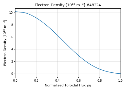
electron_density_profile · shot 48224 Stale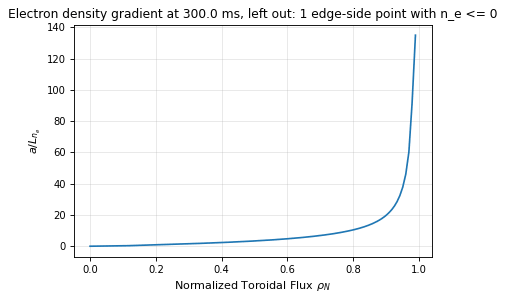
electron_density_profile_gradient · shot 48224 Stale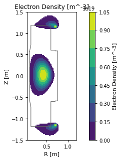
electron_density_field · shot 48224 Staleelectron_density_time
time
source
electron_density / time · domain core_profiles · view model LineSeries
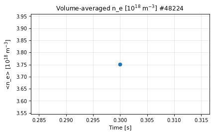
Volume-averaged electron density history.
Thumbnail drawn from sample shot 48224, stale: renderer or style changed.
vaft.omas.plot_electron_density_time(ods)         # from data
vaft.plot.electron_density_time(model)   # from a LineSeries
Show source vaft/plot/renderers/lines.py, lines 1535–1557
@renderer(
    domain="core_profiles",
    subject="electron_density",
    view="time",
    quantity="",
    model=LineSeries,
    description="Volume-averaged electron density history.",
    ids=("core_profiles",),
    required_paths=(
        "core_profiles.time",
        "core_profiles.profiles_1d.{i}.electrons.density",
    ),
    optional_paths=("core_profiles.profiles_1d.{i}.grid.volume",),
)
def electron_density_time(
    model: LineSeries,
    *,
    ax: Axes | None = None,
    show: bool = False,
    **style: Any,
) -> tuple[Figure, Axes]:
    """Volume-averaged electron density history."""
return render_line_series(model, ax=ax, show=show, **style)| IDS | core_profiles |
|---|---|
| Required paths | core_profiles.timecore_profiles.profiles_1d.{i}.electrons.density |
| Optional paths | core_profiles.profiles_1d.{i}.grid.volume |
| Backends | matplotlib, plotly |
| Renderer | vaft.plot.renderers.lines.electron_density_time |
electron_density_profile
profile
source
electron_density / profile · domain core_profiles · view model Profile1D
Core electron density profile.
Interpretation
The electron density against the radial flux coordinate at one core_profiles time. It is read for the central density, the peaking, the gradient regions and the edge, and for how the profile evolves with fuelling and confinement.
Limitations
A core_profiles entry may be a fit to measurements, a model or an assumed profile; the curve between measurement points is the fit’s, not the data. Mapping onto a flux coordinate uses an equilibrium, whose errors move the points radially.
See Also
See Also
thomson_scattering_profile_fit : the measurements behind a fitted profile. electron_density_field : the same profile mapped onto the poloidal plane.
Thumbnail drawn from sample shot 48224, stale: renderer or style changed.
vaft.omas.plot_electron_density_profile(ods)         # from data
vaft.plot.electron_density_profile(model)   # from a Profile1D
Show source vaft/plot/renderers/profiles.py, lines 504–546
@_profile_renderer(
    domain="core_profiles", quantity="",
    subject="electron_density",
    description="Core electron density profile.",
    ids=("core_profiles",),
    required_paths=("core_profiles.profiles_1d.{i}.electrons.density",),
    optional_paths=("core_profiles.profiles_1d.{i}.grid.rho_tor_norm",),
)
def electron_density_profile(
    model: Profile1D, *, ax: Axes | None = None, show: bool = False, **style: Any
) -> tuple[Figure, Axes]:
    """Core electron density profile.

    Interpretation
    --------------
    The electron density against the radial flux coordinate at one
    core_profiles time.  It is read for the central density, the peaking, the
    gradient regions and the edge, and for how the profile evolves with
    fuelling and confinement.

    Options
    -------
    ``coordinate=`` draws the profile against rho_tor_norm, the square root of
    the normalized toroidal flux, or against the normalized poloidal flux
    psi_N; the values do not change, but positions do, so
    profiles are compared on one coordinate.  ``rational_q=`` and
    ``resonances=`` mark rational surfaces from the equilibrium's q profile.
    ``uncertainty=`` and ``validity=`` control how stored uncertainties and
    flagged values are drawn.

    Limitations
    -----------
    A core_profiles entry may be a fit to measurements, a model or an assumed
    profile; the curve between measurement points is the fit's, not the data.
    Mapping onto a flux coordinate uses an equilibrium, whose errors move the
    points radially.

    See Also
    --------
    thomson_scattering_profile_fit : the measurements behind a fitted profile.
    electron_density_field : the same profile mapped onto the poloidal plane.
    """
return render_profile_1d(model, ax=ax, show=show, **style)| IDS | core_profiles |
|---|---|
| Required paths | core_profiles.profiles_1d.{i}.electrons.density |
| Optional paths | core_profiles.profiles_1d.{i}.grid.rho_tor_norm |
| Backends | matplotlib, plotly |
| Renderer | vaft.plot.renderers.profiles.electron_density_profile |
electron_density_profile_gradient
profile
source
electron_density / profile / gradient · domain core_profiles · view model Profile1D
Normalized logarithmic gradient of the core electron density, -L d ln f/dx, with its abscissa, gradient coordinate and reference length stated (a/L by default).
Thumbnail drawn from sample shot 48224, stale: renderer or style changed.
vaft.omas.plot_electron_density_profile_gradient(ods)         # from data
vaft.plot.electron_density_profile_gradient(model)   # from a Profile1D
Show source vaft/plot/renderers/profiles.py, lines 600–618
@_profile_renderer(
    domain="core_profiles", quantity="gradient",
    subject="electron_density",
    description=(
        "Normalized logarithmic gradient of the core electron density, -L d ln f/dx, with its "
        "abscissa, gradient coordinate and reference length stated (a/L by default)."
    ),
    ids=("core_profiles", "equilibrium"),
    required_paths=(
        "core_profiles.profiles_1d.{i}.electrons.density",
        *_GRADIENT_EQUILIBRIUM_PATHS,
    ),
    optional_paths=_GRADIENT_GRID_PATHS,
)
def electron_density_profile_gradient(
    model: Profile1D, *, ax: Axes | None = None, show: bool = False, **style: Any
) -> tuple[Figure, Axes]:
    """Core electron density gradient; the model carries the values, the label and the record."""
return render_profile_1d(model, ax=ax, show=show, **style)| IDS | core_profiles, equilibrium |
|---|---|
| Required paths | core_profiles.profiles_1d.{i}.electrons.densityequilibrium.time_slice.{i}.profiles_1d.psiequilibrium.time_slice.{i}.profiles_2d.{j}.psiequilibrium.time_slice.{i}.global_quantities.magnetic_axis.r |
| Optional paths | core_profiles.profiles_1d.{i}.grid.psicore_profiles.profiles_1d.{i}.grid.rho_pol_normcore_profiles.profiles_1d.{i}.grid.rho_tor_norm |
| Backends | matplotlib, plotly |
| Renderer | vaft.plot.renderers.profiles.electron_density_profile_gradient |
electron_density_field
field
source
electron_density / field · domain core_profiles · view model Field2D
Electron density mapped onto the poloidal plane.
Interpretation
The electron density profile drawn on the poloidal (R, Z) plane through the equilibrium flux surfaces: each grid cell takes the profile’s value at its own flux surface. It shows where the density sits relative to the vessel and to diagnostic and heating beam paths.
Limitations
The map holds no information beyond the 1-D profile and the equilibrium: it assumes the quantity is constant on each flux surface, so poloidal asymmetries are absent by construction. Cells are filled wherever the normalized flux is below 1 and left blank elsewhere, so a private-flux region below an X-point, or flux that recurs near a coil, is filled although it is not inside the plasma.
See Also
See Also
electron_density_profile : the 1-D profile that is mapped.
Thumbnail drawn from sample shot 48224, stale: renderer or style changed.
vaft.omas.plot_electron_density_field(ods)         # from data
vaft.plot.electron_density_field(model)   # from a Field2D
Show source vaft/plot/renderers/fields.py, lines 401–442
@_field_renderer(
    domain="core_profiles", quantity="",
    subject="electron_density",
    description="Electron density mapped onto the poloidal plane.",
    ids=("core_profiles", "equilibrium", "wall"),
    required_paths=(
        "core_profiles.profiles_1d.{i}.electrons.density",
        "equilibrium.time_slice.{i}.profiles_2d.{j}.psi",
    ),
    optional_paths=("core_profiles.profiles_1d.{i}.grid.rho_tor_norm",),
)
def electron_density_field(
    model: Field2D, *, ax: Axes | None = None, show: bool = False, **style: Any
) -> tuple[Figure, Axes]:
    """Electron density mapped onto the poloidal plane.

    Interpretation
    --------------
    The electron density profile drawn on the poloidal (R, Z) plane through the
    equilibrium flux surfaces: each grid cell takes the profile's value at its
    own flux surface.  It shows where the density sits relative to the vessel
    and to diagnostic and heating beam paths.

    Options
    -------
    ``time_slice=`` names the equilibrium slice; the profile mapped onto it is
    the core_profiles entry stored at that slice's time.

    Limitations
    -----------
    The map holds no information beyond the 1-D profile and the equilibrium: it
    assumes the quantity is constant on each flux surface, so poloidal
    asymmetries are absent by construction.  Cells are filled wherever the
    normalized flux is below 1 and left blank elsewhere, so a private-flux
    region below an X-point, or flux that recurs near a coil, is filled
    although it is not inside the plasma.

    See Also
    --------
    electron_density_profile : the 1-D profile that is mapped.
    """
return render_field_2d(model, ax=ax, show=show, **style)| IDS | core_profiles, equilibrium, wall |
|---|---|
| Required paths | core_profiles.profiles_1d.{i}.electrons.densityequilibrium.time_slice.{i}.profiles_2d.{j}.psi |
| Optional paths | core_profiles.profiles_1d.{i}.grid.rho_tor_norm |
| Backends | matplotlib, plotly |
| Renderer | vaft.plot.renderers.fields.electron_density_field |
electron_temperature [te, T_e]
electron_temperature_time · shot 48224 Stale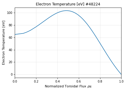
electron_temperature_profile · shot 48224 Stale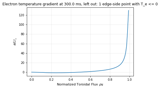
electron_temperature_profile_gradient · shot 48224 Stale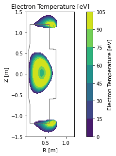
electron_temperature_field · shot 48224 Staleelectron_temperature_time
time
source
electron_temperature / time · domain core_profiles · view model LineSeries
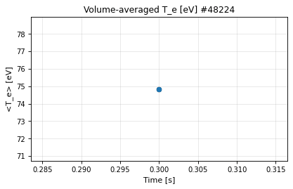
Volume-averaged electron temperature history.
Thumbnail drawn from sample shot 48224, stale: renderer or style changed.
vaft.omas.plot_electron_temperature_time(ods)         # from data
vaft.plot.electron_temperature_time(model)   # from a LineSeries
Show source vaft/plot/renderers/lines.py, lines 1510–1532
@renderer(
    domain="core_profiles",
    subject="electron_temperature",
    view="time",
    quantity="",
    model=LineSeries,
    description="Volume-averaged electron temperature history.",
    ids=("core_profiles",),
    required_paths=(
        "core_profiles.time",
        "core_profiles.profiles_1d.{i}.electrons.temperature",
    ),
    optional_paths=("core_profiles.profiles_1d.{i}.grid.volume",),
)
def electron_temperature_time(
    model: LineSeries,
    *,
    ax: Axes | None = None,
    show: bool = False,
    **style: Any,
) -> tuple[Figure, Axes]:
    """Volume-averaged electron temperature history."""
return render_line_series(model, ax=ax, show=show, **style)| IDS | core_profiles |
|---|---|
| Required paths | core_profiles.timecore_profiles.profiles_1d.{i}.electrons.temperature |
| Optional paths | core_profiles.profiles_1d.{i}.grid.volume |
| Backends | matplotlib, plotly |
| Renderer | vaft.plot.renderers.lines.electron_temperature_time |
electron_temperature_profile
profile
source
electron_temperature / profile · domain core_profiles · view model Profile1D
Core electron temperature profile.
Interpretation
The electron temperature against the radial flux coordinate at one core_profiles time. It is read for the central temperature, the peaking, the regions of steep gradient and a pedestal if there is one, and for how the profile changes between times or discharges.
Limitations
A core_profiles entry may be a fit to measurements, a model or an assumed profile; the curve between measurement points is the fit’s, not the data. Mapping onto a flux coordinate uses an equilibrium, whose errors move the points radially.
See Also
See Also
thomson_scattering_profile_fit : the measurements behind a fitted profile. electron_temperature_field : the same profile mapped onto the poloidal plane.
Thumbnail drawn from sample shot 48224, stale: renderer or style changed.
vaft.omas.plot_electron_temperature_profile(ods)         # from data
vaft.plot.electron_temperature_profile(model)   # from a Profile1D
Show source vaft/plot/renderers/profiles.py, lines 459–501
@_profile_renderer(
    domain="core_profiles", quantity="",
    subject="electron_temperature",
    description="Core electron temperature profile.",
    ids=("core_profiles",),
    required_paths=("core_profiles.profiles_1d.{i}.electrons.temperature",),
    optional_paths=("core_profiles.profiles_1d.{i}.grid.rho_tor_norm",),
)
def electron_temperature_profile(
    model: Profile1D, *, ax: Axes | None = None, show: bool = False, **style: Any
) -> tuple[Figure, Axes]:
    """Core electron temperature profile.

    Interpretation
    --------------
    The electron temperature against the radial flux coordinate at one
    core_profiles time.  It is read for the central temperature, the peaking,
    the regions of steep gradient and a pedestal if there is one, and for how
    the profile changes between times or discharges.

    Options
    -------
    ``coordinate=`` draws the profile against rho_tor_norm, the square root of
    the normalized toroidal flux, or against the normalized poloidal flux
    psi_N; the values do not change, but positions do, so
    profiles are compared on one coordinate.  ``rational_q=`` and
    ``resonances=`` mark rational surfaces from the equilibrium's q profile.
    ``uncertainty=`` and ``validity=`` control how stored uncertainties and
    flagged values are drawn.

    Limitations
    -----------
    A core_profiles entry may be a fit to measurements, a model or an assumed
    profile; the curve between measurement points is the fit's, not the data.
    Mapping onto a flux coordinate uses an equilibrium, whose errors move the
    points radially.

    See Also
    --------
    thomson_scattering_profile_fit : the measurements behind a fitted profile.
    electron_temperature_field : the same profile mapped onto the poloidal plane.
    """
return render_profile_1d(model, ax=ax, show=show, **style)| IDS | core_profiles |
|---|---|
| Required paths | core_profiles.profiles_1d.{i}.electrons.temperature |
| Optional paths | core_profiles.profiles_1d.{i}.grid.rho_tor_norm |
| Backends | matplotlib, plotly |
| Renderer | vaft.plot.renderers.profiles.electron_temperature_profile |
electron_temperature_profile_gradient
profile
source
electron_temperature / profile / gradient · domain core_profiles · view model Profile1D
Normalized logarithmic gradient of the core electron temperature, -L d ln f/dx, with its abscissa, gradient coordinate and reference length stated (a/L by default).
Thumbnail drawn from sample shot 48224, stale: renderer or style changed.
vaft.omas.plot_electron_temperature_profile_gradient(ods)         # from data
vaft.plot.electron_temperature_profile_gradient(model)   # from a Profile1D
Show source vaft/plot/renderers/profiles.py, lines 579–597
@_profile_renderer(
    domain="core_profiles", quantity="gradient",
    subject="electron_temperature",
    description=(
        "Normalized logarithmic gradient of the core electron temperature, -L d ln f/dx, with its "
        "abscissa, gradient coordinate and reference length stated (a/L by default)."
    ),
    ids=("core_profiles", "equilibrium"),
    required_paths=(
        "core_profiles.profiles_1d.{i}.electrons.temperature",
        *_GRADIENT_EQUILIBRIUM_PATHS,
    ),
    optional_paths=_GRADIENT_GRID_PATHS,
)
def electron_temperature_profile_gradient(
    model: Profile1D, *, ax: Axes | None = None, show: bool = False, **style: Any
) -> tuple[Figure, Axes]:
    """Core electron temperature gradient; the model carries the values, the label and the record."""
return render_profile_1d(model, ax=ax, show=show, **style)| IDS | core_profiles, equilibrium |
|---|---|
| Required paths | core_profiles.profiles_1d.{i}.electrons.temperatureequilibrium.time_slice.{i}.profiles_1d.psiequilibrium.time_slice.{i}.profiles_2d.{j}.psiequilibrium.time_slice.{i}.global_quantities.magnetic_axis.r |
| Optional paths | core_profiles.profiles_1d.{i}.grid.psicore_profiles.profiles_1d.{i}.grid.rho_pol_normcore_profiles.profiles_1d.{i}.grid.rho_tor_norm |
| Backends | matplotlib, plotly |
| Renderer | vaft.plot.renderers.profiles.electron_temperature_profile_gradient |
electron_temperature_field
field
source
electron_temperature / field · domain core_profiles · view model Field2D
Electron temperature mapped onto the poloidal plane.
Interpretation
The electron temperature profile drawn on the poloidal (R, Z) plane through the equilibrium flux surfaces: each grid cell takes the profile’s value at its own flux surface. It shows where the hot core sits relative to the vessel and the diagnostics’ lines of sight.
Limitations
The map holds no information beyond the 1-D profile and the equilibrium: it assumes the quantity is constant on each flux surface, so poloidal asymmetries are absent by construction. Cells are filled wherever the normalized flux is below 1 and left blank elsewhere, so a private-flux region below an X-point, or flux that recurs near a coil, is filled although it is not inside the plasma.
See Also
See Also
electron_temperature_profile : the 1-D profile that is mapped.
Thumbnail drawn from sample shot 48224, stale: renderer or style changed.
vaft.omas.plot_electron_temperature_field(ods)         # from data
vaft.plot.electron_temperature_field(model)   # from a Field2D
Show source vaft/plot/renderers/fields.py, lines 357–398
@_field_renderer(
    domain="core_profiles", quantity="",
    subject="electron_temperature",
    description="Electron temperature mapped onto the poloidal plane.",
    ids=("core_profiles", "equilibrium", "wall"),
    required_paths=(
        "core_profiles.profiles_1d.{i}.electrons.temperature",
        "equilibrium.time_slice.{i}.profiles_2d.{j}.psi",
    ),
    optional_paths=("core_profiles.profiles_1d.{i}.grid.rho_tor_norm",),
)
def electron_temperature_field(
    model: Field2D, *, ax: Axes | None = None, show: bool = False, **style: Any
) -> tuple[Figure, Axes]:
    """Electron temperature mapped onto the poloidal plane.

    Interpretation
    --------------
    The electron temperature profile drawn on the poloidal (R, Z) plane through
    the equilibrium flux surfaces: each grid cell takes the profile's value at
    its own flux surface.  It shows where the hot core sits relative to the
    vessel and the diagnostics' lines of sight.

    Options
    -------
    ``time_slice=`` names the equilibrium slice; the profile mapped onto it is
    the core_profiles entry stored at that slice's time.

    Limitations
    -----------
    The map holds no information beyond the 1-D profile and the equilibrium: it
    assumes the quantity is constant on each flux surface, so poloidal
    asymmetries are absent by construction.  Cells are filled wherever the
    normalized flux is below 1 and left blank elsewhere, so a private-flux
    region below an X-point, or flux that recurs near a coil, is filled
    although it is not inside the plasma.

    See Also
    --------
    electron_temperature_profile : the 1-D profile that is mapped.
    """
return render_field_2d(model, ax=ax, show=show, **style)| IDS | core_profiles, equilibrium, wall |
|---|---|
| Required paths | core_profiles.profiles_1d.{i}.electrons.temperatureequilibrium.time_slice.{i}.profiles_2d.{j}.psi |
| Optional paths | core_profiles.profiles_1d.{i}.grid.rho_tor_norm |
| Backends | matplotlib, plotly |
| Renderer | vaft.plot.renderers.fields.electron_temperature_field |
ion_temperature [ti, T_i]
ion_temperature_profile · shot 48224 Stale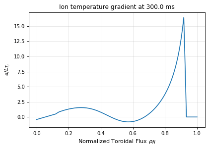
ion_temperature_profile_gradient · shot 48224 Staleion_temperature_profile
profile
source
ion_temperature / profile · domain core_profiles · view model Profile1D
Core ion temperature profile.
Thumbnail drawn from sample shot 48224, stale: renderer or style changed.
vaft.omas.plot_ion_temperature_profile(ods)         # from data
vaft.plot.ion_temperature_profile(model)   # from a Profile1D
Show source vaft/plot/renderers/profiles.py, lines 549–561
@_profile_renderer(
    domain="core_profiles", quantity="",
    subject="ion_temperature",
    description="Core ion temperature profile.",
    ids=("core_profiles",),
    required_paths=("core_profiles.profiles_1d.{i}.ion.{j}.temperature",),
    optional_paths=("core_profiles.profiles_1d.{i}.grid.rho_tor_norm",),
)
def ion_temperature_profile(
    model: Profile1D, *, ax: Axes | None = None, show: bool = False, **style: Any
) -> tuple[Figure, Axes]:
    """Core ion temperature profile."""
return render_profile_1d(model, ax=ax, show=show, **style)| IDS | core_profiles |
|---|---|
| Required paths | core_profiles.profiles_1d.{i}.ion.{j}.temperature |
| Optional paths | core_profiles.profiles_1d.{i}.grid.rho_tor_norm |
| Backends | matplotlib, plotly |
| Renderer | vaft.plot.renderers.profiles.ion_temperature_profile |
ion_temperature_profile_gradient
profile
source
ion_temperature / profile / gradient · domain core_profiles · view model Profile1D
Normalized logarithmic gradient of the core ion temperature, -L d ln f/dx, with its abscissa, gradient coordinate and reference length stated (a/L by default).
Thumbnail drawn from sample shot 48224, stale: renderer or style changed.
vaft.omas.plot_ion_temperature_profile_gradient(ods)         # from data
vaft.plot.ion_temperature_profile_gradient(model)   # from a Profile1D
Show source vaft/plot/renderers/profiles.py, lines 621–639
@_profile_renderer(
    domain="core_profiles", quantity="gradient",
    subject="ion_temperature",
    description=(
        "Normalized logarithmic gradient of the core ion temperature, -L d ln f/dx, with its "
        "abscissa, gradient coordinate and reference length stated (a/L by default)."
    ),
    ids=("core_profiles", "equilibrium"),
    required_paths=(
        "core_profiles.profiles_1d.{i}.ion.{j}.temperature",
        *_GRADIENT_EQUILIBRIUM_PATHS,
    ),
    optional_paths=_GRADIENT_GRID_PATHS,
)
def ion_temperature_profile_gradient(
    model: Profile1D, *, ax: Axes | None = None, show: bool = False, **style: Any
) -> tuple[Figure, Axes]:
    """Core ion temperature gradient; the model carries the values, the label and the record."""
return render_profile_1d(model, ax=ax, show=show, **style)| IDS | core_profiles, equilibrium |
|---|---|
| Required paths | core_profiles.profiles_1d.{i}.ion.{j}.temperatureequilibrium.time_slice.{i}.profiles_1d.psiequilibrium.time_slice.{i}.profiles_2d.{j}.psiequilibrium.time_slice.{i}.global_quantities.magnetic_axis.r |
| Optional paths | core_profiles.profiles_1d.{i}.grid.psicore_profiles.profiles_1d.{i}.grid.rho_pol_normcore_profiles.profiles_1d.{i}.grid.rho_tor_norm |
| Backends | matplotlib, plotly |
| Renderer | vaft.plot.renderers.profiles.ion_temperature_profile_gradient |
thermal_pressure [kinetic_pressure]
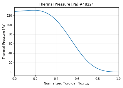
thermal_pressure_profile · shot 48224 Stalethermal_pressure_profile
profile
source
thermal_pressure / profile · domain core_profiles · view model Profile1D
Core total pressure profile.
Thumbnail drawn from sample shot 48224, stale: renderer or style changed.
vaft.omas.plot_thermal_pressure_profile(ods)         # from data
vaft.plot.thermal_pressure_profile(model)   # from a Profile1D
Show source vaft/plot/renderers/profiles.py, lines 642–654
@_profile_renderer(
    domain="core_profiles", quantity="",
    subject="thermal_pressure",
    description="Core total pressure profile.",
    ids=("core_profiles",),
    required_paths=("core_profiles.profiles_1d.{i}.pressure_thermal",),
    optional_paths=("core_profiles.profiles_1d.{i}.grid.rho_tor_norm",),
)
def thermal_pressure_profile(
    model: Profile1D, *, ax: Axes | None = None, show: bool = False, **style: Any
) -> tuple[Figure, Axes]:
    """Core total pressure profile."""
return render_profile_1d(model, ax=ax, show=show, **style)| IDS | core_profiles |
|---|---|
| Required paths | core_profiles.profiles_1d.{i}.pressure_thermal |
| Optional paths | core_profiles.profiles_1d.{i}.grid.rho_tor_norm |
| Backends | matplotlib, plotly |
| Renderer | vaft.plot.renderers.profiles.thermal_pressure_profile |
limiter_current [limiter_shunt]
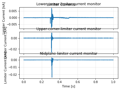
limiter_current_time · shot 39915 Stalelimiter_current_time
time
source
limiter_current / time · domain magnetics · view model Panels
Lower-corner, upper-corner and midplane limiter currents in three panels.
Thumbnail drawn from sample shot 39915, stale: renderer or style changed.
vaft.omas.plot_limiter_current_time(ods)         # from data
vaft.plot.limiter_current_time(model)   # from a Panels
Show source vaft/plot/renderers/panels.py, lines 1236–1257
@_panel_renderer(
    domain="magnetics",
    subject="limiter_current",
    view="time",
    quantity="",
    description="Lower-corner, upper-corner and midplane limiter currents in three panels.",
    ids=("magnetics",),
    required_paths=(
        "magnetics.shunt.{i}.voltage.data",
        "magnetics.shunt.{i}.resistance",
    ),
    optional_paths=(
        "magnetics.shunt.{i}.voltage.time",
        "magnetics.shunt.{i}.name",
        "magnetics.shunt.{i}.identifier",
    ),
)
def limiter_current_time(
    model: Panels, *, ax: Any = None, show: bool = False, **style: Any
) -> tuple[Figure, np.ndarray]:
    """Lower-corner, upper-corner and midplane limiter-current histories."""
return render_panels(model, ax=ax, show=show, **style)| IDS | magnetics |
|---|---|
| Required paths | magnetics.shunt.{i}.voltage.datamagnetics.shunt.{i}.resistance |
| Optional paths | magnetics.shunt.{i}.voltage.timemagnetics.shunt.{i}.namemagnetics.shunt.{i}.identifier |
| Backends | matplotlib, plotly |
| Renderer | vaft.plot.renderers.panels.limiter_current_time |
Diagnostic subjects
flux_loop
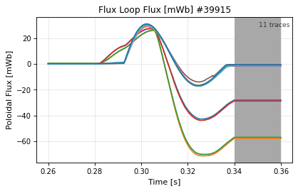
flux_loop_time_flux · shot 39915 Stale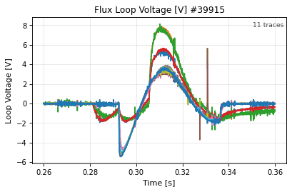
flux_loop_time_voltage · shot 39915 Stale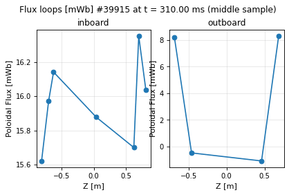
flux_loop_spatial_flux · shot 39915 Staleflux_loop_time_flux
time
source
flux_loop / time / flux · domain magnetics · view model LineSeries
Poloidal flux measured by each selected flux loop.
Interpretation
The poloidal flux linked by each flux loop against time. Flux loops sample psi at fixed points outside the plasma: their common rise follows the ohmic-coil and plasma flux, and the differences between loops carry the plasma’s position and shape. They are primary constraints of a magnetic equilibrium reconstruction, and the loop voltage is their time derivative.
Limitations
Each trace is the total flux at the loop – coils, vessel currents and
plasma together – so the plasma’s own contribution needs the vacuum
response subtracted. Integrated signals can drift, and a flagged channel
is still drawn unless validity= says otherwise.
Convention · See Also
Convention
Flux is in full weber, not weber per radian.
See Also
flux_loop_spatial_flux : the same loops against position at one time. magnetics_overview_plasma_residual : the signal left after the vacuum response.
Thumbnail drawn from sample shot 39915, stale: renderer or style changed.
vaft.omas.plot_flux_loop_time_flux(ods)         # from data
vaft.plot.flux_loop_time_flux(model)   # from a LineSeries
Show source vaft/plot/renderers/lines.py, lines 261–320
@renderer(
    domain="magnetics",
    subject="flux_loop",
    view="time",
    quantity="flux",
    model=LineSeries,
    description="Poloidal flux measured by each selected flux loop.",
    ids=("magnetics",),
    required_paths=("magnetics.flux_loop.{i}.flux.data",),
    optional_paths=(
        "magnetics.flux_loop.time",
        "magnetics.time",
        "magnetics.flux_loop.{i}.position.0.r",
        "magnetics.flux_loop.{i}.position.0.z",
    ),
)
def flux_loop_time_flux(
    model: LineSeries,
    *,
    ax: Axes | None = None,
    show: bool = False,
    **style: Any,
) -> tuple[Figure, Axes]:
    """Poloidal flux measured by each selected flux loop.

    Interpretation
    --------------
    The poloidal flux linked by each flux loop against time.  Flux loops sample
    psi at fixed points outside the plasma: their common rise follows the
    ohmic-coil and plasma flux, and the differences between loops carry the
    plasma's position and shape.  They are primary constraints of a magnetic
    equilibrium reconstruction, and the loop voltage is their time derivative.

    Options
    -------
    ``selection=`` / ``channels=`` choose the sensors and ``layout=`` whether
    they share one axes or are split into panels or groups.  ``validity=``
    decides what happens to channels the data flag as invalid: drawn but
    demoted (the default, so a reader sees them), removed, or treated as valid.
    ``synthetic=`` overlays, as markers at each equilibrium slice, the value
    the reconstruction predicts for this signal, so measurement and fit can be
    compared where the fit exists.

    Convention
    ----------
    Flux is in full weber, not weber per radian.

    Limitations
    -----------
    Each trace is the total flux at the loop -- coils, vessel currents and
    plasma together -- so the plasma's own contribution needs the vacuum
    response subtracted.  Integrated signals can drift, and a flagged channel
    is still drawn unless ``validity=`` says otherwise.

    See Also
    --------
    flux_loop_spatial_flux : the same loops against position at one time.
    magnetics_overview_plasma_residual : the signal left after the vacuum response.
    """
return render_line_series(model, ax=ax, show=show, **style)| IDS | magnetics |
|---|---|
| Required paths | magnetics.flux_loop.{i}.flux.data |
| Optional paths | magnetics.flux_loop.timemagnetics.timemagnetics.flux_loop.{i}.position.0.rmagnetics.flux_loop.{i}.position.0.z |
| Backends | matplotlib, plotly |
| Renderer | vaft.plot.renderers.lines.flux_loop_time_flux |
flux_loop_time_voltage
time
source
flux_loop / time / voltage · domain magnetics · view model LineSeries
Loop voltage measured by each selected flux loop.
Interpretation
The voltage induced in each flux loop, the rate of change of the poloidal flux it links. It shows the inductive drive applied to the plasma – the breakdown voltage, the ramp-up and flat-top loop voltage – and its spatial variation between loops.
Limitations
The voltage at a loop is not the voltage at the plasma surface or on axis, and it contains the inductive change of the plasma’s own flux; the resistive part needs the inductive correction.
See Also
See Also
flux_loop_time_flux : the integrated flux of the same loops. summary_time_voltage_consumption : resistive and inductive flux consumption.
Thumbnail drawn from sample shot 39915, stale: renderer or style changed.
vaft.omas.plot_flux_loop_time_voltage(ods)         # from data
vaft.plot.flux_loop_time_voltage(model)   # from a LineSeries
Show source vaft/plot/renderers/lines.py, lines 323–371
@renderer(
    domain="magnetics",
    subject="flux_loop",
    view="time",
    quantity="voltage",
    model=LineSeries,
    description="Loop voltage measured by each selected flux loop.",
    ids=("magnetics",),
    required_paths=("magnetics.flux_loop.{i}.voltage.data",),
    optional_paths=(
        "magnetics.flux_loop.time",
        "magnetics.time",
    ),
)
def flux_loop_time_voltage(
    model: LineSeries,
    *,
    ax: Axes | None = None,
    show: bool = False,
    **style: Any,
) -> tuple[Figure, Axes]:
    """Loop voltage measured by each selected flux loop.

    Interpretation
    --------------
    The voltage induced in each flux loop, the rate of change of the poloidal
    flux it links.  It shows the inductive drive applied to the plasma -- the
    breakdown voltage, the ramp-up and flat-top loop voltage -- and its spatial
    variation between loops.

    Options
    -------
    ``selection=`` / ``channels=`` choose the sensors and ``layout=`` whether
    they share one axes or are split into panels or groups.  ``validity=``
    decides what happens to channels the data flag as invalid: drawn but
    demoted (the default, so a reader sees them), removed, or treated as valid.

    Limitations
    -----------
    The voltage at a loop is not the voltage at the plasma surface or on axis,
    and it contains the inductive change of the plasma's own flux; the
    resistive part needs the inductive correction.

    See Also
    --------
    flux_loop_time_flux : the integrated flux of the same loops.
    summary_time_voltage_consumption : resistive and inductive flux consumption.
    """
return render_line_series(model, ax=ax, show=show, **style)| IDS | magnetics |
|---|---|
| Required paths | magnetics.flux_loop.{i}.voltage.data |
| Optional paths | magnetics.flux_loop.timemagnetics.time |
| Backends | matplotlib, plotly |
| Renderer | vaft.plot.renderers.lines.flux_loop_time_voltage |
flux_loop_spatial_flux
spatial
source
flux_loop / spatial / flux · domain magnetics · view model Profile1D
Flux-loop flux against sensor position at one time: height (inboard and outboard panels) or poloidal angle about the layout centre.
Interpretation
The flux of every loop at one instant, against where the loop sits. It shows the spatial pattern behind the time traces: an up-down asymmetry can reflect a vertical plasma displacement or asymmetric coil currents, an inboard-outboard difference the radial position and current.
Limitations
The values include the vacuum field. Sensors are sparse: whatever is drawn between them is not measured.
See Also
See Also
flux_loop_time_flux : the same loops against time.
Thumbnail drawn from sample shot 39915, stale: renderer or style changed.
vaft.omas.plot_flux_loop_spatial_flux(ods)         # from data
vaft.plot.flux_loop_spatial_flux(model)   # from a Profile1D
Show source vaft/plot/renderers/profiles.py, lines 175–213
@renderer(
    domain="magnetics",
    subject="flux_loop",
    view="spatial",
    quantity="flux",
    model=Profile1D,
    description="Flux-loop flux against sensor position at one time: height (inboard and outboard panels) or poloidal angle about the layout centre.",
    ids=("magnetics",),
    required_paths=("magnetics.flux_loop.{i}.flux.data",),
    optional_paths=_SENSOR_POSITIONS["flux_loop"] + ("magnetics.flux_loop.{i}.flux.time", "magnetics.time"),
)
def flux_loop_spatial_flux(model: Profile1D, *, ax: Axes | None = None, show: bool = False, **style: Any) -> tuple[Figure, Axes]:
    """Flux-loop flux against sensor position at one time (issue #486).

    Interpretation
    --------------
    The flux of every loop at one instant, against where the loop sits.  It
    shows the spatial pattern behind the time traces: an up-down asymmetry can
    reflect a vertical plasma displacement or asymmetric coil currents, an
    inboard-outboard difference the radial position and current.

    Options
    -------
    ``time=`` picks the stored sample nearest the requested instant; nothing is
    interpolated.  ``coordinate=`` draws the sensors either against height,
    with inboard and outboard sensors in separate panels, or against their
    poloidal angle about the centre of the sensor layout (``centre=`` moves
    it). ``validity=`` treats flagged channels as in the time view.

    Limitations
    -----------
    The values include the vacuum field.  Sensors are sparse: whatever is drawn
    between them is not measured.

    See Also
    --------
    flux_loop_time_flux : the same loops against time.
    """
return render_profile_1d(model, ax=ax, show=show, **style)| IDS | magnetics |
|---|---|
| Required paths | magnetics.flux_loop.{i}.flux.data |
| Optional paths | magnetics.flux_loop.{i}.position.0.rmagnetics.flux_loop.{i}.position.0.zmagnetics.flux_loop.{i}.flux.timemagnetics.time |
| Backends | matplotlib, plotly |
| Renderer | vaft.plot.renderers.profiles.flux_loop_spatial_flux |
b_field_probe [b_pol_probe, bpol_probe]
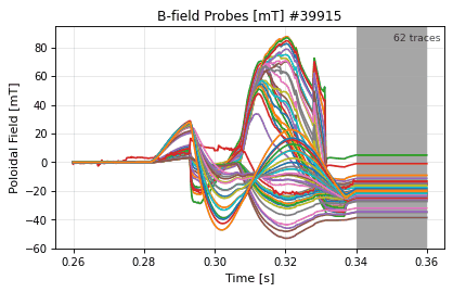
b_field_probe_time_field · shot 39915 Stale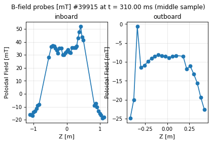
b_field_probe_spatial_field · shot 39915 Staleb_field_probe_time_field
time
source
b_field_probe / time / field · domain magnetics · view model LineSeries
Poloidal field measured by each selected B-field probe.
Interpretation
The poloidal field each magnetic probe measures along its own orientation, against time. Probes around the vessel sample the field at the boundary of the plasma region, which depends on the plasma current, its position and the current distribution; they are, with the flux loops, the main constraints of a magnetic reconstruction.
Limitations
Each probe measures one component, along its axis, of the total field – coils, vessel currents and plasma together. Probe signals are integrated from induced voltages and can drift.
See Also
See Also
b_field_probe_spatial_field : the same probes against position at one time. mirnov_spectrogram : the fluctuating part of the probe signals.
Thumbnail drawn from sample shot 39915, stale: renderer or style changed.
vaft.omas.plot_b_field_probe_time_field(ods)         # from data
vaft.plot.b_field_probe_time_field(model)   # from a LineSeries
Show source vaft/plot/renderers/lines.py, lines 374–428
@renderer(
    domain="magnetics",
    subject="b_field_probe",
    view="time",
    quantity="field",
    model=LineSeries,
    description="Poloidal field measured by each selected B-field probe.",
    ids=("magnetics",),
    required_paths=("magnetics.b_field_pol_probe.{i}.field.data",),
    optional_paths=(
        "magnetics.b_field_pol_probe.time",
        "magnetics.time",
        "magnetics.b_field_pol_probe.{i}.position.r",
        "magnetics.b_field_pol_probe.{i}.position.z",
    ),
)
def b_field_probe_time_field(
    model: LineSeries,
    *,
    ax: Axes | None = None,
    show: bool = False,
    **style: Any,
) -> tuple[Figure, Axes]:
    """Poloidal field measured by each selected B-field probe.

    Interpretation
    --------------
    The poloidal field each magnetic probe measures along its own orientation,
    against time.  Probes around the vessel sample the field at the boundary of
    the plasma region, which depends on the plasma current, its position and
    the current distribution; they are, with the flux loops, the main
    constraints of a magnetic reconstruction.

    Options
    -------
    ``selection=`` / ``channels=`` choose the sensors and ``layout=`` whether
    they share one axes or are split into panels or groups.  ``validity=``
    decides what happens to channels the data flag as invalid: drawn but
    demoted (the default, so a reader sees them), removed, or treated as valid.
    ``synthetic=`` overlays, as markers at each equilibrium slice, the value
    the reconstruction predicts for this signal, so measurement and fit can be
    compared where the fit exists.

    Limitations
    -----------
    Each probe measures one component, along its axis, of the total field --
    coils, vessel currents and plasma together.  Probe signals are integrated
    from induced voltages and can drift.

    See Also
    --------
    b_field_probe_spatial_field : the same probes against position at one time.
    mirnov_spectrogram : the fluctuating part of the probe signals.
    """
return render_line_series(model, ax=ax, show=show, **style)| IDS | magnetics |
|---|---|
| Required paths | magnetics.b_field_pol_probe.{i}.field.data |
| Optional paths | magnetics.b_field_pol_probe.timemagnetics.timemagnetics.b_field_pol_probe.{i}.position.rmagnetics.b_field_pol_probe.{i}.position.z |
| Backends | matplotlib, plotly |
| Renderer | vaft.plot.renderers.lines.b_field_probe_time_field |
b_field_probe_spatial_field
spatial
source
b_field_probe / spatial / field · domain magnetics · view model Profile1D
B-probe field against sensor position at one time: height (inboard and outboard panels) or poloidal angle about the layout centre.
Interpretation
The field of every magnetic probe at one instant, against where the probe sits. It shows how the poloidal field is distributed around the plasma region at that time, which follows the plasma’s position, shape and current distribution as well as the coil field.
Limitations
Each probe measures one field component along its own axis, so neighbouring probes mounted differently are not directly comparable. The values include the vacuum field, and nothing between sensors is measured.
See Also
See Also
b_field_probe_time_field : the same probes against time.
Thumbnail drawn from sample shot 39915, stale: renderer or style changed.
vaft.omas.plot_b_field_probe_spatial_field(ods)         # from data
vaft.plot.b_field_probe_spatial_field(model)   # from a Profile1D
Show source vaft/plot/renderers/profiles.py, lines 216–256
@renderer(
    domain="magnetics",
    subject="b_field_probe",
    view="spatial",
    quantity="field",
    model=Profile1D,
    description="B-probe field against sensor position at one time: height (inboard and outboard panels) or poloidal angle about the layout centre.",
    ids=("magnetics",),
    required_paths=("magnetics.b_field_pol_probe.{i}.field.data",),
    optional_paths=_SENSOR_POSITIONS["b_field_probe"] + ("magnetics.b_field_pol_probe.{i}.field.time", "magnetics.time"),
)
def b_field_probe_spatial_field(model: Profile1D, *, ax: Axes | None = None, show: bool = False, **style: Any) -> tuple[Figure, Axes]:
    """B-probe poloidal field against sensor position at one time (issue #486).

    Interpretation
    --------------
    The field of every magnetic probe at one instant, against where the probe
    sits.  It shows how the poloidal field is distributed around the plasma
    region at that time, which follows the plasma's position, shape and current
    distribution as well as the coil field.

    Options
    -------
    ``time=`` picks the stored sample nearest the requested instant; nothing is
    interpolated.  ``coordinate=`` draws the sensors either against height,
    with inboard and outboard sensors in separate panels, or against their
    poloidal angle about the centre of the sensor layout (``centre=`` moves
    it). ``validity=`` treats flagged channels as in the time view. ``angle=``
    chooses the geometric poloidal angle or the one stored with each probe.

    Limitations
    -----------
    Each probe measures one field component along its own axis, so neighbouring
    probes mounted differently are not directly comparable.  The values include
    the vacuum field, and nothing between sensors is measured.

    See Also
    --------
    b_field_probe_time_field : the same probes against time.
    """
return render_profile_1d(model, ax=ax, show=show, **style)| IDS | magnetics |
|---|---|
| Required paths | magnetics.b_field_pol_probe.{i}.field.data |
| Optional paths | magnetics.b_field_pol_probe.{i}.position.rmagnetics.b_field_pol_probe.{i}.position.zmagnetics.b_field_pol_probe.{i}.poloidal_anglemagnetics.b_field_pol_probe.{i}.field.timemagnetics.time |
| Backends | matplotlib, plotly |
| Renderer | vaft.plot.renderers.profiles.b_field_probe_spatial_field |
mirnov [mirnov_coil]
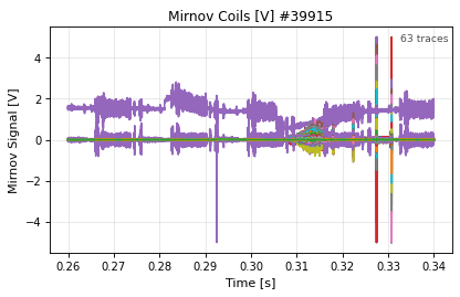
mirnov_time_voltage · shot 39915 Stale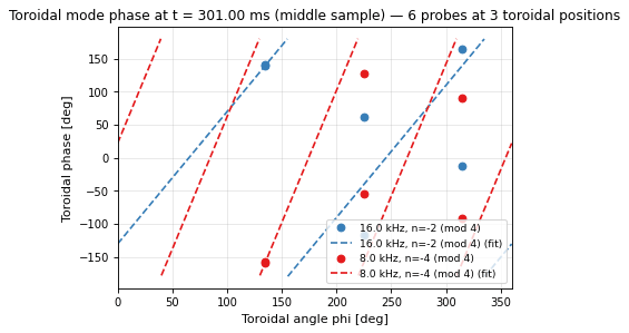
mirnov_spatial_phase · shot 45531 Stale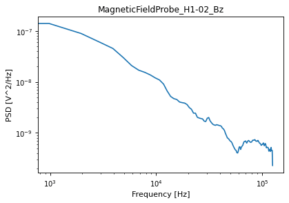
mirnov_spectrum · shot 39915 Stale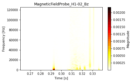
mirnov_spectrogram · shot 39915 Stalemirnov_time_voltage
time
source
mirnov / time / voltage · domain magnetics · view model LineSeries
Raw or preprocessed Mirnov coil voltage traces.
Interpretation
The voltage induced in each Mirnov coil, proportional to the rate of change of the field through it. The traces show when MHD activity, sawtooth-like crashes or other fast magnetic events happen and how strongly each coil responds, before any spectral analysis.
Limitations
A coil voltage weights each frequency by that frequency, so a fast mode looks stronger than a slow one of equal field amplitude. Slow equilibrium changes and pickup also appear, and comparing amplitudes between coils requires their effective areas. The traces are as raw or as preprocessed as the stored signal.
See Also
See Also
mirnov_spectrogram : the frequency content of one coil against time. mirnov_spatial_phase : toroidal phase across the coils, for mode numbers.
Thumbnail drawn from sample shot 39915, stale: renderer or style changed.
vaft.omas.plot_mirnov_time_voltage(ods)         # from data
vaft.plot.mirnov_time_voltage(model)   # from a LineSeries
Show source vaft/plot/renderers/lines.py, lines 482–530
@renderer(
    domain="magnetics",
    subject="mirnov",
    view="time",
    quantity="voltage",
    model=LineSeries,
    description="Raw or preprocessed Mirnov coil voltage traces.",
    ids=("magnetics",),
    required_paths=("magnetics.b_field_pol_probe.{i}.voltage.data",),
    optional_paths=(
        "magnetics.b_field_pol_probe.{i}.voltage.time",
        "magnetics.time",
    ),
)
def mirnov_time_voltage(
    model: LineSeries,
    *,
    ax: Axes | None = None,
    show: bool = False,
    **style: Any,
) -> tuple[Figure, Axes]:
    """Raw or preprocessed Mirnov coil voltage traces.

    Interpretation
    --------------
    The voltage induced in each Mirnov coil, proportional to the rate of change
    of the field through it.  The traces show when MHD activity, sawtooth-like
    crashes or other fast magnetic events happen and how strongly each coil
    responds, before any spectral analysis.

    Options
    -------
    ``selection=`` / ``channels=`` choose the coils and ``layout=`` how they
    are arranged.

    Limitations
    -----------
    A coil voltage weights each frequency by that frequency, so a fast mode
    looks stronger than a slow one of equal field amplitude.  Slow equilibrium
    changes and pickup also appear, and comparing amplitudes between coils
    requires their effective areas.  The traces are as raw or as preprocessed
    as the stored signal.

    See Also
    --------
    mirnov_spectrogram : the frequency content of one coil against time.
    mirnov_spatial_phase : toroidal phase across the coils, for mode numbers.
    """
return render_line_series(model, ax=ax, show=show, **style)| IDS | magnetics |
|---|---|
| Required paths | magnetics.b_field_pol_probe.{i}.voltage.data |
| Optional paths | magnetics.b_field_pol_probe.{i}.voltage.timemagnetics.time |
| Backends | matplotlib, plotly |
| Renderer | vaft.plot.renderers.lines.mirnov_time_voltage |
mirnov_spatial_phase
spatial
source
mirnov / spatial / phase · domain magnetics · view model Profile1D
Toroidal phase of each fluctuation band around the torus at one time, with the fitted n mode lines.
Thumbnail drawn from sample shot 45531, stale: renderer or style changed.
vaft.omas.plot_mirnov_spatial_phase(ods)         # from data
vaft.plot.mirnov_spatial_phase(model)   # from a Profile1D
Show source vaft/plot/renderers/profiles.py, lines 155–172
@renderer(
    domain="magnetics",
    subject="mirnov",
    view="spatial",
    quantity="phase",
    model=Profile1D,
    description="Toroidal phase of each fluctuation band around the torus at one time, with the fitted n mode lines.",
    ids=("magnetics",),
    required_paths=("magnetics.b_field_pol_probe.{i}.voltage.data",),
    optional_paths=(
        "magnetics.b_field_pol_probe.{i}.position.phi",
        "magnetics.b_field_pol_probe.{i}.voltage.time",
        "magnetics.time",
    ),
)
def mirnov_spatial_phase(model: Profile1D, *, ax: Axes | None = None, show: bool = False, **style: Any) -> tuple[Figure, Axes]:
    """Toroidal phase per fluctuation band at one time (issue #485)."""
return render_profile_1d(model, ax=ax, show=show, **style)| IDS | magnetics |
|---|---|
| Required paths | magnetics.b_field_pol_probe.{i}.voltage.data |
| Optional paths | magnetics.b_field_pol_probe.{i}.position.phimagnetics.b_field_pol_probe.{i}.voltage.timemagnetics.time |
| Backends | matplotlib, plotly |
| Renderer | vaft.plot.renderers.profiles.mirnov_spatial_phase |
mirnov_spectrum
spectrum
source
mirnov / spectrum · domain magnetics · view model PowerSpectrum
Power spectral density of one Mirnov coil signal.
Thumbnail drawn from sample shot 39915, stale: renderer or style changed.
vaft.omas.plot_mirnov_spectrum(ods)         # from data
vaft.plot.mirnov_spectrum(model)   # from a PowerSpectrum
Show source vaft/plot/renderers/spectra.py, lines 138–153
@renderer(
    domain="magnetics",
    subject="mirnov",
    view="spectrum",
    quantity="",
    model=PowerSpectrum,
    description="Power spectral density of one Mirnov coil signal.",
    ids=("magnetics",),
    required_paths=("magnetics.b_field_pol_probe.{i}.voltage.data",),
    optional_paths=("magnetics.b_field_pol_probe.{i}.voltage.time", "magnetics.time"),
)
def mirnov_spectrum(
    model: PowerSpectrum, *, ax: Axes | None = None, show: bool = False, **style: Any
) -> tuple[Figure, Axes]:
    """Power spectral density of one Mirnov coil signal."""
return render_power_spectrum(model, ax=ax, show=show, **style)| IDS | magnetics |
|---|---|
| Required paths | magnetics.b_field_pol_probe.{i}.voltage.data |
| Optional paths | magnetics.b_field_pol_probe.{i}.voltage.timemagnetics.time |
| Backends | matplotlib |
| Renderer | vaft.plot.renderers.spectra.mirnov_spectrum |
mirnov_spectrogram
spectrogram
source
mirnov / spectrogram · domain magnetics · view model Spectrogram
Time-frequency map of one Mirnov coil signal.
Interpretation
The spectral magnitude of one Mirnov coil’s voltage in sliding windows. A coherent MHD mode appears as a narrow band, and its frequency history shows onset, frequency chirping as rotation changes, and locking when the band drops to zero frequency and vanishes; broadband activity and crashes appear as vertical stripes.
Limitations
One coil gives no mode numbers: identifying m and n needs the phase across an array. The coil voltage is a time derivative, so higher frequencies are emphasized. The observed frequency is in the laboratory frame and includes the plasma rotation’s Doppler shift, so it is not the mode frequency in the plasma frame. A narrow band can also be pickup or aliasing.
See Also
See Also
mirnov_time_voltage : the coil signals themselves. mirnov_spatial_phase : toroidal phase per band, for the mode number n.
Thumbnail drawn from sample shot 39915, stale: renderer or style changed.
vaft.omas.plot_mirnov_spectrogram(ods)         # from data
vaft.plot.mirnov_spectrogram(model)   # from a Spectrogram
Show source vaft/plot/renderers/spectrograms.py, lines 108–155
@renderer(
    domain="magnetics",
    subject="mirnov",
    view="spectrogram",
    quantity="",
    model=Spectrogram,
    description="Time-frequency map of one Mirnov coil signal.",
    ids=("magnetics",),
    required_paths=("magnetics.b_field_pol_probe.{i}.voltage.data",),
    optional_paths=("magnetics.b_field_pol_probe.{i}.voltage.time", "magnetics.time"),
)
def mirnov_spectrogram(
    model: Spectrogram, *, ax: Axes | None = None, show: bool = False, **style: Any
) -> tuple[Figure, Axes]:
    """Time-frequency map of one Mirnov coil signal.

    Interpretation
    --------------
    The spectral magnitude of one Mirnov coil's voltage in sliding windows.  A
    coherent MHD mode appears as a narrow band, and its frequency history shows
    onset, frequency chirping as rotation changes, and locking when the band
    drops to zero frequency and vanishes; broadband activity and crashes appear
    as vertical stripes.

    Options
    -------
    ``method=`` chooses the transform: a short-time Fourier transform, the
    Hann-window FFT the VEST Mirnov analyses were written against, or a
    continuous wavelet, whose resolution varies with frequency and which needs
    a named ``frequency_range=``.  Window length trades time against frequency
    resolution.  ``frequency_range=`` names the analysis band.  ``track=``
    overlays the ridge of the dominant frequency in a band, with ``max_jump=``
    limiting how far it may move between windows.

    Limitations
    -----------
    One coil gives no mode numbers: identifying m and n needs the phase across
    an array.  The coil voltage is a time derivative, so higher frequencies are
    emphasized.  The observed frequency is in the laboratory frame and includes
    the plasma rotation's Doppler shift, so it is not the mode frequency in the
    plasma frame.  A narrow band can also be pickup or aliasing.

    See Also
    --------
    mirnov_time_voltage : the coil signals themselves.
    mirnov_spatial_phase : toroidal phase per band, for the mode number n.
    """
return render_spectrogram(model, ax=ax, show=show, **style)| IDS | magnetics |
|---|---|
| Required paths | magnetics.b_field_pol_probe.{i}.voltage.data |
| Optional paths | magnetics.b_field_pol_probe.{i}.voltage.timemagnetics.time |
| Backends | matplotlib, plotly |
| Renderer | vaft.plot.renderers.spectrograms.mirnov_spectrogram |
impa [hall_probe_array]
impa_time_fieldimpa_time_voltageimpa_profile_field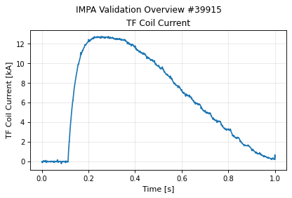
impa_overview · shot 39915 Staleimpa_time_field
time
source
impa / time / field · domain magnetics · view model LineSeries
Calibrated field from the IMPA Hall-probe array.
No thumbnail: no packaged sample carries the data this plot needs.
vaft.omas.plot_impa_time_field(ods)         # from data
vaft.plot.impa_time_field(model)   # from a LineSeries
Show source vaft/plot/renderers/lines.py, lines 431–454
@renderer(
    domain="magnetics",
    subject="impa",
    view="time",
    quantity="field",
    model=LineSeries,
    description="Calibrated field from the IMPA Hall-probe array.",
    ids=("magnetics",),
    required_paths=("magnetics.b_field_tor_probe.{i}.field.data",),
    optional_paths=(
        "magnetics.b_field_tor_probe.{i}.identifier",
        "magnetics.b_field_tor_probe.{i}.position.r",
        "magnetics.b_field_pol_probe.{i}.field.data",
    ),
)
def impa_time_field(
    model: LineSeries,
    *,
    ax: Axes | None = None,
    show: bool = False,
    **style: Any,
) -> tuple[Figure, Axes]:
    """Calibrated field from the IMPA Hall-probe array."""
return render_line_series(model, ax=ax, show=show, **style)| IDS | magnetics |
|---|---|
| Required paths | magnetics.b_field_tor_probe.{i}.field.data |
| Optional paths | magnetics.b_field_tor_probe.{i}.identifiermagnetics.b_field_tor_probe.{i}.position.rmagnetics.b_field_pol_probe.{i}.field.data |
| Backends | matplotlib, plotly |
| Renderer | vaft.plot.renderers.lines.impa_time_field |
impa_time_voltage
time
source
impa / time / voltage · domain magnetics · view model LineSeries
Raw IMPA Hall-probe voltages, one trace per channel.
No thumbnail: no packaged sample carries the data this plot needs.
vaft.omas.plot_impa_time_voltage(ods)         # from data
vaft.plot.impa_time_voltage(model)   # from a LineSeries
Show source vaft/plot/renderers/lines.py, lines 457–479
@renderer(
    domain="magnetics",
    subject="impa",
    view="time",
    quantity="voltage",
    model=LineSeries,
    description="Raw IMPA Hall-probe voltages, one trace per channel.",
    ids=("magnetics",),
    required_paths=("magnetics.b_field_tor_probe.{i}.voltage.data",),
    optional_paths=(
        "magnetics.b_field_tor_probe.{i}.identifier",
        "magnetics.b_field_pol_probe.{i}.voltage.data",
    ),
)
def impa_time_voltage(
    model: LineSeries,
    *,
    ax: Axes | None = None,
    show: bool = False,
    **style: Any,
) -> tuple[Figure, Axes]:
    """Raw IMPA Hall-probe voltages."""
return render_line_series(model, ax=ax, show=show, **style)| IDS | magnetics |
|---|---|
| Required paths | magnetics.b_field_tor_probe.{i}.voltage.data |
| Optional paths | magnetics.b_field_tor_probe.{i}.identifiermagnetics.b_field_pol_probe.{i}.voltage.data |
| Backends | matplotlib, plotly |
| Renderer | vaft.plot.renderers.lines.impa_time_voltage |
impa_profile_field
profile
source
impa / profile / field · domain magnetics · view model Profile1D
IMPA measured field against probe radius with the 1/R toroidal-field model.
No thumbnail: no packaged sample carries the data this plot needs.
vaft.omas.plot_impa_profile_field(ods)         # from data
vaft.plot.impa_profile_field(model)   # from a Profile1D
Show source vaft/plot/renderers/profiles.py, lines 782–806
@renderer(
    domain="magnetics",
    subject="impa",
    view="profile",
    quantity="field",
    model=Profile1D,
    description="IMPA measured field against probe radius with the 1/R toroidal-field model.",
    ids=("magnetics", "tf"),
    required_paths=("magnetics.b_field_tor_probe.{i}.voltage.data",),
    optional_paths=(
        "magnetics.b_field_tor_probe.{i}.identifier",
        "magnetics.b_field_tor_probe.{i}.position.r",
        "magnetics.b_field_pol_probe.{i}.voltage.data",
        "tf.coil.{i}.current.data",
    ),
)
def impa_profile_field(
    model: Profile1D,
    *,
    ax: Axes | None = None,
    show: bool = False,
    **style: Any,
) -> tuple[Figure, Axes]:
    """IMPA radial profile against the 1/R toroidal-field model."""
return render_profile_1d(model, ax=ax, show=show, **style)| IDS | magnetics, tf |
|---|---|
| Required paths | magnetics.b_field_tor_probe.{i}.voltage.data |
| Optional paths | magnetics.b_field_tor_probe.{i}.identifiermagnetics.b_field_tor_probe.{i}.position.rmagnetics.b_field_pol_probe.{i}.voltage.datatf.coil.{i}.current.data |
| Backends | matplotlib, plotly |
| Renderer | vaft.plot.renderers.profiles.impa_profile_field |
impa_overview
overview
source
impa / overview · domain magnetics · view model Panels
IMPA validation overview: raw voltages, compensated Bz and the 1/R position check.
Thumbnail drawn from sample shot 39915, stale: renderer or style changed.
vaft.omas.plot_impa_overview(ods)         # from data
vaft.plot.impa_overview(model)   # from a Panels
Show source vaft/plot/renderers/panels.py, lines 1222–1233
@_panel_renderer(
    domain="magnetics", view="overview", quantity="",
    subject="impa",
    description="IMPA validation overview: raw voltages, compensated Bz and the 1/R position check.",
    ids=("magnetics", "tf"),
    required_paths=("magnetics.b_field_tor_probe.{i}.voltage.data",),
)
def impa_overview(
    model: Panels, *, ax: Any = None, show: bool = False, **style: Any
) -> tuple[Figure, np.ndarray]:
    """IMPA validation overview panels."""
return render_panels(model, ax=ax, show=show, **style)| IDS | magnetics, tf |
|---|---|
| Required paths | magnetics.b_field_tor_probe.{i}.voltage.data |
| Backends | matplotlib, plotly |
| Renderer | vaft.plot.renderers.panels.impa_overview |
soft_x_rays [soft_x_ray, sxr]
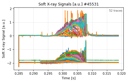
soft_x_rays_time_power · shot 45531 Stale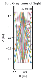
soft_x_rays_geometry_lines_of_sight · shot 45531 Stale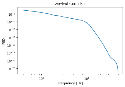
soft_x_rays_spectrum · shot 45531 Stale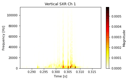
soft_x_rays_spectrogram · shot 45531 Stale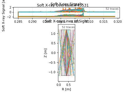
soft_x_rays_overview · shot 45531 Stalesoft_x_rays_time_power
time
source
soft_x_rays / time / power · domain soft_x_rays · view model LineSeries
Soft X-ray channel signal history.
Thumbnail drawn from sample shot 45531, stale: renderer or style changed.
vaft.omas.plot_soft_x_rays_time_power(ods)         # from data
vaft.plot.soft_x_rays_time_power(model)   # from a LineSeries
Show source vaft/plot/renderers/lines.py, lines 1354–1379
@renderer(
    domain="soft_x_rays",
    subject="soft_x_rays",
    view="time",
    quantity="power",
    model=LineSeries,
    description="Soft X-ray channel signal history.",
    ids=("soft_x_rays",),
    required_paths=("soft_x_rays.channel.{i}.brightness.data",),
    optional_paths=(
        "soft_x_rays.channel.{i}.brightness.time",
        "soft_x_rays.channel.{i}.power.data",
        "soft_x_rays.channel.{i}.power.time",
        "soft_x_rays.time",
        "soft_x_rays.channel.{i}.name",
    ),
)
def soft_x_rays_time_power(
    model: LineSeries,
    *,
    ax: Axes | None = None,
    show: bool = False,
    **style: Any,
) -> tuple[Figure, Axes]:
    """Soft X-ray channel signal history."""
return render_line_series(model, ax=ax, show=show, **style)| IDS | soft_x_rays |
|---|---|
| Required paths | soft_x_rays.channel.{i}.brightness.data |
| Optional paths | soft_x_rays.channel.{i}.brightness.timesoft_x_rays.channel.{i}.power.datasoft_x_rays.channel.{i}.power.timesoft_x_rays.timesoft_x_rays.channel.{i}.name |
| Backends | matplotlib, plotly |
| Renderer | vaft.plot.renderers.lines.soft_x_rays_time_power |
soft_x_rays_geometry_lines_of_sight
geometry
source
soft_x_rays / geometry / lines_of_sight · domain soft_x_rays · view model GeometryLayers
Soft X-ray detector lines of sight over the poloidal cross-section.
Thumbnail drawn from sample shot 45531, stale: renderer or style changed.
vaft.omas.plot_soft_x_rays_geometry_lines_of_sight(ods)         # from data
vaft.plot.soft_x_rays_geometry_lines_of_sight(model)   # from a GeometryLayers
Show source vaft/plot/renderers/geometry.py, lines 362–377
@_geometry_renderer(
    domain="soft_x_rays", quantity="lines_of_sight",
    subject="soft_x_rays",
    description="Soft X-ray detector lines of sight over the poloidal cross-section.",
    ids=("soft_x_rays", "wall"),
    required_paths=("soft_x_rays.channel.{i}.line_of_sight.first_point.r",
                    "soft_x_rays.channel.{i}.line_of_sight.first_point.z",
                    "soft_x_rays.channel.{i}.line_of_sight.second_point.r",
                    "soft_x_rays.channel.{i}.line_of_sight.second_point.z"),
    optional_paths=("wall.description_2d.{i}.limiter.unit.{j}.outline.r",),
)
def soft_x_rays_geometry_lines_of_sight(
    model: GeometryLayers, *, ax: Axes | None = None, show: bool = False, **style: Any
) -> tuple[Figure, Axes]:
    """Soft X-ray detector lines of sight over the poloidal cross-section."""
return render_geometry_layers(model, ax=ax, show=show, **style)| IDS | soft_x_rays, wall |
|---|---|
| Required paths | soft_x_rays.channel.{i}.line_of_sight.first_point.rsoft_x_rays.channel.{i}.line_of_sight.first_point.zsoft_x_rays.channel.{i}.line_of_sight.second_point.rsoft_x_rays.channel.{i}.line_of_sight.second_point.z |
| Optional paths | wall.description_2d.{i}.limiter.unit.{j}.outline.r |
| Backends | matplotlib |
| Renderer | vaft.plot.renderers.geometry.soft_x_rays_geometry_lines_of_sight |
soft_x_rays_spectrum
spectrum
source
soft_x_rays / spectrum · domain soft_x_rays · view model PowerSpectrum
Power spectral density of one soft X-ray channel.
Thumbnail drawn from sample shot 45531, stale: renderer or style changed.
vaft.omas.plot_soft_x_rays_spectrum(ods)         # from data
vaft.plot.soft_x_rays_spectrum(model)   # from a PowerSpectrum
Show source vaft/plot/renderers/spectra.py, lines 156–175
@renderer(
    domain="soft_x_rays",
    subject="soft_x_rays",
    view="spectrum",
    model=PowerSpectrum,
    description="Power spectral density of one soft X-ray channel.",
    ids=("soft_x_rays",),
    required_paths=("soft_x_rays.channel.{i}.brightness.data",),
    optional_paths=(
        "soft_x_rays.channel.{i}.brightness.time",
        "soft_x_rays.channel.{i}.power.data",
        "soft_x_rays.channel.{i}.power.time",
        "soft_x_rays.time",
    ),
)
def soft_x_rays_spectrum(
    model: PowerSpectrum, *, ax: Axes | None = None, show: bool = False, **style: Any
) -> tuple[Figure, Axes]:
    """Power spectral density of one soft X-ray channel."""
return render_power_spectrum(model, ax=ax, show=show, **style)| IDS | soft_x_rays |
|---|---|
| Required paths | soft_x_rays.channel.{i}.brightness.data |
| Optional paths | soft_x_rays.channel.{i}.brightness.timesoft_x_rays.channel.{i}.power.datasoft_x_rays.channel.{i}.power.timesoft_x_rays.time |
| Backends | matplotlib |
| Renderer | vaft.plot.renderers.spectra.soft_x_rays_spectrum |
soft_x_rays_spectrogram
spectrogram
source
soft_x_rays / spectrogram · domain soft_x_rays · view model Spectrogram
Time-frequency map of one soft X-ray channel.
Thumbnail drawn from sample shot 45531, stale: renderer or style changed.
vaft.omas.plot_soft_x_rays_spectrogram(ods)         # from data
vaft.plot.soft_x_rays_spectrogram(model)   # from a Spectrogram
Show source vaft/plot/renderers/spectrograms.py, lines 158–177
@renderer(
    domain="soft_x_rays",
    subject="soft_x_rays",
    view="spectrogram",
    model=Spectrogram,
    description="Time-frequency map of one soft X-ray channel.",
    ids=("soft_x_rays",),
    required_paths=("soft_x_rays.channel.{i}.brightness.data",),
    optional_paths=(
        "soft_x_rays.channel.{i}.brightness.time",
        "soft_x_rays.channel.{i}.power.data",
        "soft_x_rays.channel.{i}.power.time",
        "soft_x_rays.time",
    ),
)
def soft_x_rays_spectrogram(
    model: Spectrogram, *, ax: Axes | None = None, show: bool = False, **style: Any
) -> tuple[Figure, Axes]:
    """Time-frequency map of one soft X-ray channel."""
return render_spectrogram(model, ax=ax, show=show, **style)| IDS | soft_x_rays |
|---|---|
| Required paths | soft_x_rays.channel.{i}.brightness.data |
| Optional paths | soft_x_rays.channel.{i}.brightness.timesoft_x_rays.channel.{i}.power.datasoft_x_rays.channel.{i}.power.timesoft_x_rays.time |
| Backends | matplotlib, plotly |
| Renderer | vaft.plot.renderers.spectrograms.soft_x_rays_spectrogram |
soft_x_rays_overview
overview
source
soft_x_rays / overview / channels · domain soft_x_rays · view model Panels
Soft X-ray overview: lines of sight, signals and channel pattern.
Thumbnail drawn from sample shot 45531, stale: renderer or style changed.
vaft.omas.plot_soft_x_rays_overview(ods)         # from data
vaft.plot.soft_x_rays_overview(model)   # from a Panels
Show source vaft/plot/renderers/panels.py, lines 1717–1731
@_panel_renderer(
    domain="soft_x_rays",
    subject="soft_x_rays",
    view="overview",
    quantity="channels",
    description="Soft X-ray overview: lines of sight, signals and channel pattern.",
    ids=("soft_x_rays", "wall"),
    required_paths=("soft_x_rays.channel.{i}.brightness.data",),
    optional_paths=("soft_x_rays.channel.{i}.power.data",),
)
def soft_x_rays_overview(
    model: Panels, *, ax: Any = None, show: bool = False, **style: Any
) -> tuple[Figure, np.ndarray]:
    """Soft X-ray overview panels."""
return render_panels(model, ax=ax, show=show, **style)| IDS | soft_x_rays, wall |
|---|---|
| Required paths | soft_x_rays.channel.{i}.brightness.data |
| Optional paths | soft_x_rays.channel.{i}.power.data |
| Backends | matplotlib, plotly |
| Renderer | vaft.plot.renderers.panels.soft_x_rays_overview |
interferometer
interferometer_time_n_e_lineinterferometer_spectruminterferometer_spectrograminterferometer_overviewinterferometer_time_n_e_line
time
source
interferometer / time / n_e_line · domain interferometer · view model LineSeries
Interferometer line-integrated electron density history.
No thumbnail: no packaged sample carries the data this plot needs.
vaft.omas.plot_interferometer_time_n_e_line(ods)         # from data
vaft.plot.interferometer_time_n_e_line(model)   # from a LineSeries
Show source vaft/plot/renderers/lines.py, lines 1382–1405
@renderer(
    domain="interferometer",
    subject="interferometer",
    view="time",
    quantity="n_e_line",
    model=LineSeries,
    description="Interferometer line-integrated electron density history.",
    ids=("interferometer",),
    required_paths=("interferometer.channel.{i}.n_e_line.data",),
    optional_paths=(
        "interferometer.channel.{i}.n_e_line.time",
        "interferometer.time",
        "interferometer.channel.{i}.name",
    ),
)
def interferometer_time_n_e_line(
    model: LineSeries,
    *,
    ax: Axes | None = None,
    show: bool = False,
    **style: Any,
) -> tuple[Figure, Axes]:
    """Interferometer line-integrated electron density history."""
return render_line_series(model, ax=ax, show=show, **style)| IDS | interferometer |
|---|---|
| Required paths | interferometer.channel.{i}.n_e_line.data |
| Optional paths | interferometer.channel.{i}.n_e_line.timeinterferometer.timeinterferometer.channel.{i}.name |
| Backends | matplotlib, plotly |
| Renderer | vaft.plot.renderers.lines.interferometer_time_n_e_line |
interferometer_spectrum
spectrum
source
interferometer / spectrum · domain interferometer · view model PowerSpectrum
Power spectral density of one interferometer channel's line density.
No thumbnail: no packaged sample carries the data this plot needs.
vaft.omas.plot_interferometer_spectrum(ods)         # from data
vaft.plot.interferometer_spectrum(model)   # from a PowerSpectrum
Show source vaft/plot/renderers/spectra.py, lines 178–192
@renderer(
    domain="interferometer",
    subject="interferometer",
    view="spectrum",
    model=PowerSpectrum,
    description="Power spectral density of one interferometer channel's line density.",
    ids=("interferometer",),
    required_paths=("interferometer.channel.{i}.n_e_line.data",),
    optional_paths=("interferometer.channel.{i}.n_e_line.time", "interferometer.time"),
)
def interferometer_spectrum(
    model: PowerSpectrum, *, ax: Axes | None = None, show: bool = False, **style: Any
) -> tuple[Figure, Axes]:
    """Power spectral density of one interferometer channel's line density."""
return render_power_spectrum(model, ax=ax, show=show, **style)| IDS | interferometer |
|---|---|
| Required paths | interferometer.channel.{i}.n_e_line.data |
| Optional paths | interferometer.channel.{i}.n_e_line.timeinterferometer.time |
| Backends | matplotlib |
| Renderer | vaft.plot.renderers.spectra.interferometer_spectrum |
interferometer_spectrogram
spectrogram
source
interferometer / spectrogram · domain interferometer · view model Spectrogram
Time-frequency map of one interferometer channel's line density.
No thumbnail: no packaged sample carries the data this plot needs.
vaft.omas.plot_interferometer_spectrogram(ods)         # from data
vaft.plot.interferometer_spectrogram(model)   # from a Spectrogram
Show source vaft/plot/renderers/spectrograms.py, lines 180–194
@renderer(
    domain="interferometer",
    subject="interferometer",
    view="spectrogram",
    model=Spectrogram,
    description="Time-frequency map of one interferometer channel's line density.",
    ids=("interferometer",),
    required_paths=("interferometer.channel.{i}.n_e_line.data",),
    optional_paths=("interferometer.channel.{i}.n_e_line.time", "interferometer.time"),
)
def interferometer_spectrogram(
    model: Spectrogram, *, ax: Axes | None = None, show: bool = False, **style: Any
) -> tuple[Figure, Axes]:
    """Time-frequency map of one interferometer channel's line density."""
return render_spectrogram(model, ax=ax, show=show, **style)| IDS | interferometer |
|---|---|
| Required paths | interferometer.channel.{i}.n_e_line.data |
| Optional paths | interferometer.channel.{i}.n_e_line.timeinterferometer.time |
| Backends | matplotlib, plotly |
| Renderer | vaft.plot.renderers.spectrograms.interferometer_spectrogram |
interferometer_overview
overview
source
interferometer / overview / channels · domain interferometer · view model Panels
Interferometer overview: line density history and spectrogram.
No thumbnail: no packaged sample carries the data this plot needs.
vaft.omas.plot_interferometer_overview(ods)         # from data
vaft.plot.interferometer_overview(model)   # from a Panels
Show source vaft/plot/renderers/panels.py, lines 1734–1745
@_panel_renderer(
    domain="interferometer", view="overview", quantity="channels",
    subject="interferometer",
    description="Interferometer overview: line density history and spectrogram.",
    ids=("interferometer",),
    required_paths=("interferometer.channel.{i}.n_e_line.data",),
)
def interferometer_overview(
    model: Panels, *, ax: Any = None, show: bool = False, **style: Any
) -> tuple[Figure, np.ndarray]:
    """Interferometer overview panels."""
return render_panels(model, ax=ax, show=show, **style)| IDS | interferometer |
|---|---|
| Required paths | interferometer.channel.{i}.n_e_line.data |
| Backends | matplotlib, plotly |
| Renderer | vaft.plot.renderers.panels.interferometer_overview |
thomson_scattering [thomson]
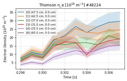
thomson_scattering_time_electron_density · shot 48224 Stale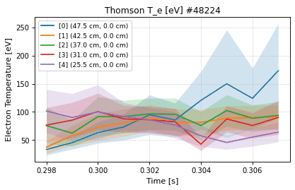
thomson_scattering_time_electron_temperature · shot 48224 Stale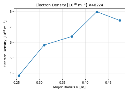
thomson_scattering_profile_electron_density · shot 48224 Stale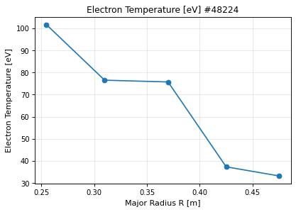
thomson_scattering_profile_electron_temperature · shot 48224 Stale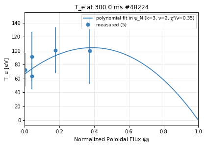
thomson_scattering_profile_fit · shot 48224 Stale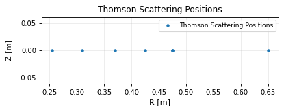
thomson_scattering_geometry_poloidal · shot 48224 Stalethomson_scattering_time_electron_density
time
source
thomson_scattering / time / electron_density · domain thomson_scattering · view model LineSeries
Per-channel Thomson electron density history.
Thumbnail drawn from sample shot 48224, stale: renderer or style changed.
vaft.omas.plot_thomson_scattering_time_electron_density(ods)         # from data
vaft.plot.thomson_scattering_time_electron_density(model)   # from a LineSeries
Show source vaft/plot/renderers/lines.py, lines 1433–1455
@renderer(
    domain="thomson_scattering",
    subject="thomson_scattering",
    view="time",
    quantity="electron_density",
    model=LineSeries,
    description="Per-channel Thomson electron density history.",
    ids=("thomson_scattering",),
    required_paths=(
        "thomson_scattering.time",
        "thomson_scattering.channel.{i}.n_e.data",
    ),
    optional_paths=("thomson_scattering.channel.{i}.name",),
)
def thomson_scattering_time_electron_density(
    model: LineSeries,
    *,
    ax: Axes | None = None,
    show: bool = False,
    **style: Any,
) -> tuple[Figure, Axes]:
    """Per-channel Thomson electron density history."""
return render_line_series(model, ax=ax, show=show, **style)| IDS | thomson_scattering |
|---|---|
| Required paths | thomson_scattering.timethomson_scattering.channel.{i}.n_e.data |
| Optional paths | thomson_scattering.channel.{i}.name |
| Backends | matplotlib, plotly |
| Renderer | vaft.plot.renderers.lines.thomson_scattering_time_electron_density |
thomson_scattering_time_electron_temperature
time
source
thomson_scattering / time / electron_temperature · domain thomson_scattering · view model LineSeries
Per-channel Thomson electron temperature history.
Thumbnail drawn from sample shot 48224, stale: renderer or style changed.
vaft.omas.plot_thomson_scattering_time_electron_temperature(ods)         # from data
vaft.plot.thomson_scattering_time_electron_temperature(model)   # from a LineSeries
Show source vaft/plot/renderers/lines.py, lines 1408–1430
@renderer(
    domain="thomson_scattering",
    subject="thomson_scattering",
    view="time",
    quantity="electron_temperature",
    model=LineSeries,
    description="Per-channel Thomson electron temperature history.",
    ids=("thomson_scattering",),
    required_paths=(
        "thomson_scattering.time",
        "thomson_scattering.channel.{i}.t_e.data",
    ),
    optional_paths=("thomson_scattering.channel.{i}.name",),
)
def thomson_scattering_time_electron_temperature(
    model: LineSeries,
    *,
    ax: Axes | None = None,
    show: bool = False,
    **style: Any,
) -> tuple[Figure, Axes]:
    """Per-channel Thomson electron temperature history."""
return render_line_series(model, ax=ax, show=show, **style)| IDS | thomson_scattering |
|---|---|
| Required paths | thomson_scattering.timethomson_scattering.channel.{i}.t_e.data |
| Optional paths | thomson_scattering.channel.{i}.name |
| Backends | matplotlib, plotly |
| Renderer | vaft.plot.renderers.lines.thomson_scattering_time_electron_temperature |
thomson_scattering_profile_electron_density
profile
source
thomson_scattering / profile / electron_density · domain thomson_scattering · view model Profile1D
Thomson-scattering electron density versus position.
Thumbnail drawn from sample shot 48224, stale: renderer or style changed.
vaft.omas.plot_thomson_scattering_profile_electron_density(ods)         # from data
vaft.plot.thomson_scattering_profile_electron_density(model)   # from a Profile1D
Show source vaft/plot/renderers/profiles.py, lines 675–690
@_profile_renderer(
    domain="thomson_scattering", quantity="electron_density",
    subject="thomson_scattering",
    description="Thomson-scattering electron density versus position.",
    ids=("thomson_scattering",),
    required_paths=(
        "thomson_scattering.channel.{i}.n_e.data",
        "thomson_scattering.channel.{i}.position.r",
    ),
    optional_paths=("thomson_scattering.time",),
)
def thomson_scattering_profile_electron_density(
    model: Profile1D, *, ax: Axes | None = None, show: bool = False, **style: Any
) -> tuple[Figure, Axes]:
    """Thomson-scattering electron density versus position."""
return render_profile_1d(model, ax=ax, show=show, **style)| IDS | thomson_scattering |
|---|---|
| Required paths | thomson_scattering.channel.{i}.n_e.datathomson_scattering.channel.{i}.position.r |
| Optional paths | thomson_scattering.time |
| Backends | matplotlib, plotly |
| Renderer | vaft.plot.renderers.profiles.thomson_scattering_profile_electron_density |
thomson_scattering_profile_electron_temperature
profile
source
thomson_scattering / profile / electron_temperature · domain thomson_scattering · view model Profile1D
Thomson-scattering electron temperature versus position.
Thumbnail drawn from sample shot 48224, stale: renderer or style changed.
vaft.omas.plot_thomson_scattering_profile_electron_temperature(ods)         # from data
vaft.plot.thomson_scattering_profile_electron_temperature(model)   # from a Profile1D
Show source vaft/plot/renderers/profiles.py, lines 657–672
@_profile_renderer(
    domain="thomson_scattering", quantity="electron_temperature",
    subject="thomson_scattering",
    description="Thomson-scattering electron temperature versus position.",
    ids=("thomson_scattering",),
    required_paths=(
        "thomson_scattering.channel.{i}.t_e.data",
        "thomson_scattering.channel.{i}.position.r",
    ),
    optional_paths=("thomson_scattering.time",),
)
def thomson_scattering_profile_electron_temperature(
    model: Profile1D, *, ax: Axes | None = None, show: bool = False, **style: Any
) -> tuple[Figure, Axes]:
    """Thomson-scattering electron temperature versus position."""
return render_profile_1d(model, ax=ax, show=show, **style)| IDS | thomson_scattering |
|---|---|
| Required paths | thomson_scattering.channel.{i}.t_e.datathomson_scattering.channel.{i}.position.r |
| Optional paths | thomson_scattering.time |
| Backends | matplotlib, plotly |
| Renderer | vaft.plot.renderers.profiles.thomson_scattering_profile_electron_temperature |
thomson_scattering_profile_fit
profile
source
thomson_scattering / profile / fit · domain thomson_scattering · view model Profile1D
| Thomson T_e or n_e (field=te | ne) at one time: channels with error bars, refused channels hollow, and the fit through them on psi_N, rho_N or R, mapped through the ODS's own or a given equilibrium (issue #952). |
Thumbnail drawn from sample shot 48224, stale: renderer or style changed.
vaft.omas.plot_thomson_scattering_profile_fit(ods)         # from data
vaft.plot.thomson_scattering_profile_fit(model)   # from a Profile1D
Show source vaft/plot/renderers/profiles.py, lines 693–717
@_profile_renderer(
    domain="thomson_scattering", quantity="fit",
    subject="thomson_scattering",
    description=(
        "Thomson T_e or n_e (field=te|ne) at one time: channels with error bars, refused "
        "channels hollow, and the fit through them on psi_N, rho_N or R, mapped through "
        "the ODS's own or a given equilibrium (issue #952)."
    ),
    ids=("thomson_scattering", "equilibrium"),
    required_paths=(
        "thomson_scattering.time",
        "thomson_scattering.channel.{i}.t_e.data",
        "thomson_scattering.channel.{i}.n_e.data",
        "thomson_scattering.channel.{i}.position.r",
    ),
    optional_paths=(
        "thomson_scattering.channel.{i}.t_e.data_error_upper",
        "equilibrium.time_slice.{i}.profiles_2d.{j}.psi",
    ),
)
def thomson_scattering_profile_fit(
    model: Profile1D, *, ax: Axes | None = None, show: bool = False, **style: Any
) -> tuple[Figure, Axes]:
    """Thomson points and their fit on a flux coordinate."""
return render_profile_1d(model, ax=ax, show=show, **style)| IDS | thomson_scattering, equilibrium |
|---|---|
| Required paths | thomson_scattering.timethomson_scattering.channel.{i}.t_e.datathomson_scattering.channel.{i}.n_e.datathomson_scattering.channel.{i}.position.r |
| Optional paths | thomson_scattering.channel.{i}.t_e.data_error_upperequilibrium.time_slice.{i}.profiles_2d.{j}.psi |
| Backends | matplotlib, plotly |
| Renderer | vaft.plot.renderers.profiles.thomson_scattering_profile_fit |
thomson_scattering_geometry_poloidal
geometry
source
thomson_scattering / geometry / poloidal · domain thomson_scattering · view model GeometryLayers
Thomson-scattering measurement positions in the poloidal plane.
Thumbnail drawn from sample shot 48224, stale: renderer or style changed.
vaft.omas.plot_thomson_scattering_geometry_poloidal(ods)         # from data
vaft.plot.thomson_scattering_geometry_poloidal(model)   # from a GeometryLayers
Show source vaft/plot/renderers/geometry.py, lines 380–392
@_geometry_renderer(
    domain="thomson_scattering", quantity="poloidal",
    subject="thomson_scattering",
    description="Thomson-scattering measurement positions in the poloidal plane.",
    ids=("thomson_scattering",),
    required_paths=("thomson_scattering.channel.{i}.position.r",
                    "thomson_scattering.channel.{i}.position.z"),
)
def thomson_scattering_geometry_poloidal(
    model: GeometryLayers, *, ax: Axes | None = None, show: bool = False, **style: Any
) -> tuple[Figure, Axes]:
    """Thomson-scattering measurement positions in the poloidal plane."""
return render_geometry_layers(model, ax=ax, show=show, **style)| IDS | thomson_scattering |
|---|---|
| Required paths | thomson_scattering.channel.{i}.position.rthomson_scattering.channel.{i}.position.z |
| Backends | matplotlib |
| Renderer | vaft.plot.renderers.geometry.thomson_scattering_geometry_poloidal |
charge_exchange
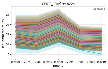
charge_exchange_time_ion_temperature · shot 48224 Stale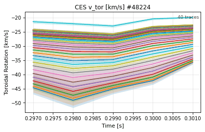
charge_exchange_time_velocity_tor · shot 48224 Stale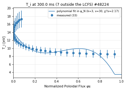
charge_exchange_profile_fit · shot 48224 Stale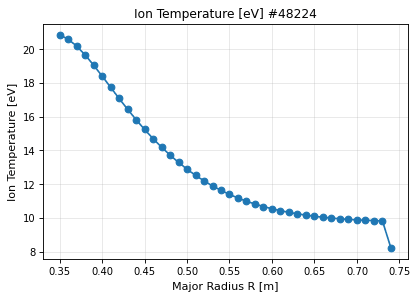
charge_exchange_profile_ion_temperature · shot 48224 Stale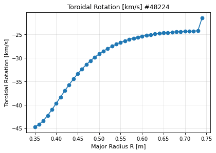
charge_exchange_profile_velocity_tor · shot 48224 Stale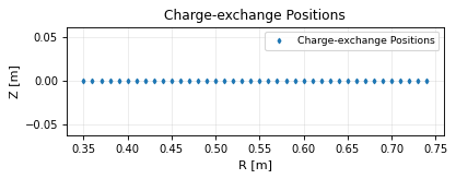
charge_exchange_geometry_poloidal · shot 48224 Stalecharge_exchange_time_ion_temperature
time
source
charge_exchange / time / ion_temperature · domain charge_exchange · view model LineSeries
Per-channel ion temperature history from charge-exchange spectroscopy.
Thumbnail drawn from sample shot 48224, stale: renderer or style changed.
vaft.omas.plot_charge_exchange_time_ion_temperature(ods)         # from data
vaft.plot.charge_exchange_time_ion_temperature(model)   # from a LineSeries
Show source vaft/plot/renderers/lines.py, lines 1458–1481
@renderer(
    domain="charge_exchange",
    subject="charge_exchange",
    view="time",
    quantity="ion_temperature",
    model=LineSeries,
    description="Per-channel ion temperature history from charge-exchange spectroscopy.",
    ids=("charge_exchange",),
    required_paths=("charge_exchange.channel.{i}.ion.{j}.t_i.data",),
    optional_paths=(
        "charge_exchange.channel.{i}.ion.{j}.t_i.time",
        "charge_exchange.time",
        "charge_exchange.channel.{i}.name",
    ),
)
def charge_exchange_time_ion_temperature(
    model: LineSeries,
    *,
    ax: Axes | None = None,
    show: bool = False,
    **style: Any,
) -> tuple[Figure, Axes]:
    """Per-channel ion temperature history from charge-exchange spectroscopy."""
return render_line_series(model, ax=ax, show=show, **style)| IDS | charge_exchange |
|---|---|
| Required paths | charge_exchange.channel.{i}.ion.{j}.t_i.data |
| Optional paths | charge_exchange.channel.{i}.ion.{j}.t_i.timecharge_exchange.timecharge_exchange.channel.{i}.name |
| Backends | matplotlib, plotly |
| Renderer | vaft.plot.renderers.lines.charge_exchange_time_ion_temperature |
charge_exchange_time_velocity_tor
time
source
charge_exchange / time / velocity_tor · domain charge_exchange · view model LineSeries
Per-channel toroidal rotation history from charge-exchange spectroscopy.
Thumbnail drawn from sample shot 48224, stale: renderer or style changed.
vaft.omas.plot_charge_exchange_time_velocity_tor(ods)         # from data
vaft.plot.charge_exchange_time_velocity_tor(model)   # from a LineSeries
Show source vaft/plot/renderers/lines.py, lines 1484–1507
@renderer(
    domain="charge_exchange",
    subject="charge_exchange",
    view="time",
    quantity="velocity_tor",
    model=LineSeries,
    description="Per-channel toroidal rotation history from charge-exchange spectroscopy.",
    ids=("charge_exchange",),
    required_paths=("charge_exchange.channel.{i}.ion.{j}.velocity_tor.data",),
    optional_paths=(
        "charge_exchange.channel.{i}.ion.{j}.velocity_tor.time",
        "charge_exchange.time",
        "charge_exchange.channel.{i}.name",
    ),
)
def charge_exchange_time_velocity_tor(
    model: LineSeries,
    *,
    ax: Axes | None = None,
    show: bool = False,
    **style: Any,
) -> tuple[Figure, Axes]:
    """Per-channel toroidal rotation history from charge-exchange spectroscopy."""
return render_line_series(model, ax=ax, show=show, **style)| IDS | charge_exchange |
|---|---|
| Required paths | charge_exchange.channel.{i}.ion.{j}.velocity_tor.data |
| Optional paths | charge_exchange.channel.{i}.ion.{j}.velocity_tor.timecharge_exchange.timecharge_exchange.channel.{i}.name |
| Backends | matplotlib, plotly |
| Renderer | vaft.plot.renderers.lines.charge_exchange_time_velocity_tor |
charge_exchange_profile_fit
profile
source
charge_exchange / profile / fit · domain charge_exchange · view model Profile1D
| Charge-exchange T_i or V_phi (field=ti | vphi) at one time: channels with error bars, refused channels hollow, and the fit through them on psi_N, rho_N or R (issue #952). |
Thumbnail drawn from sample shot 48224, stale: renderer or style changed.
vaft.omas.plot_charge_exchange_profile_fit(ods)         # from data
vaft.plot.charge_exchange_profile_fit(model)   # from a Profile1D
Show source vaft/plot/renderers/profiles.py, lines 720–743
@_profile_renderer(
    domain="charge_exchange", quantity="fit",
    subject="charge_exchange",
    description=(
        "Charge-exchange T_i or V_phi (field=ti|vphi) at one time: channels with error "
        "bars, refused channels hollow, and the fit through them on psi_N, rho_N or R "
        "(issue #952)."
    ),
    ids=("charge_exchange", "equilibrium"),
    required_paths=(
        "charge_exchange.time",
        "charge_exchange.channel.{i}.ion.{j}.t_i.data",
        "charge_exchange.channel.{i}.position.r.data",
    ),
    optional_paths=(
        "charge_exchange.channel.{i}.ion.{j}.velocity_tor.data",
        "equilibrium.time_slice.{i}.profiles_2d.{j}.psi",
    ),
)
def charge_exchange_profile_fit(
    model: Profile1D, *, ax: Axes | None = None, show: bool = False, **style: Any
) -> tuple[Figure, Axes]:
    """Charge-exchange points and their fit on a flux coordinate."""
return render_profile_1d(model, ax=ax, show=show, **style)| IDS | charge_exchange, equilibrium |
|---|---|
| Required paths | charge_exchange.timecharge_exchange.channel.{i}.ion.{j}.t_i.datacharge_exchange.channel.{i}.position.r.data |
| Optional paths | charge_exchange.channel.{i}.ion.{j}.velocity_tor.dataequilibrium.time_slice.{i}.profiles_2d.{j}.psi |
| Backends | matplotlib, plotly |
| Renderer | vaft.plot.renderers.profiles.charge_exchange_profile_fit |
charge_exchange_profile_ion_temperature
profile
source
charge_exchange / profile / ion_temperature · domain charge_exchange · view model Profile1D
Charge-exchange ion temperature versus position.
Thumbnail drawn from sample shot 48224, stale: renderer or style changed.
vaft.omas.plot_charge_exchange_profile_ion_temperature(ods)         # from data
vaft.plot.charge_exchange_profile_ion_temperature(model)   # from a Profile1D
Show source vaft/plot/renderers/profiles.py, lines 746–761
@_profile_renderer(
    domain="charge_exchange", quantity="ion_temperature",
    subject="charge_exchange",
    description="Charge-exchange ion temperature versus position.",
    ids=("charge_exchange",),
    required_paths=(
        "charge_exchange.channel.{i}.ion.{j}.t_i.data",
        "charge_exchange.channel.{i}.position.r.data",
    ),
    optional_paths=("charge_exchange.time",),
)
def charge_exchange_profile_ion_temperature(
    model: Profile1D, *, ax: Axes | None = None, show: bool = False, **style: Any
) -> tuple[Figure, Axes]:
    """Charge-exchange ion temperature versus position."""
return render_profile_1d(model, ax=ax, show=show, **style)| IDS | charge_exchange |
|---|---|
| Required paths | charge_exchange.channel.{i}.ion.{j}.t_i.datacharge_exchange.channel.{i}.position.r.data |
| Optional paths | charge_exchange.time |
| Backends | matplotlib, plotly |
| Renderer | vaft.plot.renderers.profiles.charge_exchange_profile_ion_temperature |
charge_exchange_profile_velocity_tor
profile
source
charge_exchange / profile / velocity_tor · domain charge_exchange · view model Profile1D
Charge-exchange toroidal rotation versus position.
Thumbnail drawn from sample shot 48224, stale: renderer or style changed.
vaft.omas.plot_charge_exchange_profile_velocity_tor(ods)         # from data
vaft.plot.charge_exchange_profile_velocity_tor(model)   # from a Profile1D
Show source vaft/plot/renderers/profiles.py, lines 764–779
@_profile_renderer(
    domain="charge_exchange", quantity="velocity_tor",
    subject="charge_exchange",
    description="Charge-exchange toroidal rotation versus position.",
    ids=("charge_exchange",),
    required_paths=(
        "charge_exchange.channel.{i}.ion.{j}.velocity_tor.data",
        "charge_exchange.channel.{i}.position.r.data",
    ),
    optional_paths=("charge_exchange.time",),
)
def charge_exchange_profile_velocity_tor(
    model: Profile1D, *, ax: Axes | None = None, show: bool = False, **style: Any
) -> tuple[Figure, Axes]:
    """Charge-exchange toroidal rotation versus position."""
return render_profile_1d(model, ax=ax, show=show, **style)| IDS | charge_exchange |
|---|---|
| Required paths | charge_exchange.channel.{i}.ion.{j}.velocity_tor.datacharge_exchange.channel.{i}.position.r.data |
| Optional paths | charge_exchange.time |
| Backends | matplotlib, plotly |
| Renderer | vaft.plot.renderers.profiles.charge_exchange_profile_velocity_tor |
charge_exchange_geometry_poloidal
geometry
source
charge_exchange / geometry / poloidal · domain charge_exchange · view model GeometryLayers
Charge-exchange measurement positions in the poloidal plane.
Thumbnail drawn from sample shot 48224, stale: renderer or style changed.
vaft.omas.plot_charge_exchange_geometry_poloidal(ods)         # from data
vaft.plot.charge_exchange_geometry_poloidal(model)   # from a GeometryLayers
Show source vaft/plot/renderers/geometry.py, lines 395–407
@_geometry_renderer(
    domain="charge_exchange", quantity="poloidal",
    subject="charge_exchange",
    description="Charge-exchange measurement positions in the poloidal plane.",
    ids=("charge_exchange",),
    required_paths=("charge_exchange.channel.{i}.position.r.data",
                    "charge_exchange.channel.{i}.position.z.data"),
)
def charge_exchange_geometry_poloidal(
    model: GeometryLayers, *, ax: Axes | None = None, show: bool = False, **style: Any
) -> tuple[Figure, Axes]:
    """Charge-exchange measurement positions in the poloidal plane."""
return render_geometry_layers(model, ax=ax, show=show, **style)| IDS | charge_exchange |
|---|---|
| Required paths | charge_exchange.channel.{i}.position.r.datacharge_exchange.channel.{i}.position.z.data |
| Backends | matplotlib |
| Renderer | vaft.plot.renderers.geometry.charge_exchange_geometry_poloidal |
spectrometer_uv
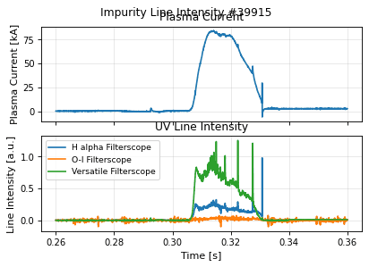
spectrometer_uv_time_impurity · shot 39915 Stale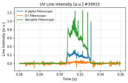
spectrometer_uv_time_intensity · shot 39915 Stalespectrometer_uv_time_impurity
time
source
spectrometer_uv / time / impurity · domain spectrometer_uv · view model Panels
Impurity line-intensity panels against plasma current.
Thumbnail drawn from sample shot 39915, stale: renderer or style changed.
vaft.omas.plot_spectrometer_uv_time_impurity(ods)         # from data
vaft.plot.spectrometer_uv_time_impurity(model)   # from a Panels
Show source vaft/plot/renderers/panels.py, lines 928–941
@_panel_renderer(
    domain="spectrometer_uv",
    subject="spectrometer_uv",
    view="time",
    quantity="impurity",
    description="Impurity line-intensity panels against plasma current.",
    ids=("spectrometer_uv", "magnetics"),
    required_paths=("spectrometer_uv.time",),
)
def spectrometer_uv_time_impurity(
    model: Panels, *, ax: Any = None, show: bool = False, **style: Any
) -> tuple[Figure, np.ndarray]:
    """Impurity line-intensity panels against plasma current."""
return render_panels(model, ax=ax, show=show, **style)| IDS | spectrometer_uv, magnetics |
|---|---|
| Required paths | spectrometer_uv.time |
| Backends | matplotlib, plotly |
| Renderer | vaft.plot.renderers.panels.spectrometer_uv_time_impurity |
spectrometer_uv_time_intensity
time
source
spectrometer_uv / time / intensity · domain spectrometer_uv · view model LineSeries
Processed spectral line intensity history.
Thumbnail drawn from sample shot 39915, stale: renderer or style changed.
vaft.omas.plot_spectrometer_uv_time_intensity(ods)         # from data
vaft.plot.spectrometer_uv_time_intensity(model)   # from a LineSeries
Show source vaft/plot/renderers/lines.py, lines 1224–1246
@renderer(
    domain="spectrometer_uv",
    subject="spectrometer_uv",
    view="time",
    quantity="intensity",
    model=LineSeries,
    description="Processed spectral line intensity history.",
    ids=("spectrometer_uv",),
    required_paths=(
        "spectrometer_uv.time",
        "spectrometer_uv.channel.{i}.processed_line.{j}.intensity.data",
    ),
    optional_paths=("spectrometer_uv.channel.{i}.processed_line.{j}.label",),
)
def spectrometer_uv_time_intensity(
    model: LineSeries,
    *,
    ax: Axes | None = None,
    show: bool = False,
    **style: Any,
) -> tuple[Figure, Axes]:
    """Processed spectral line intensity history."""
return render_line_series(model, ax=ax, show=show, **style)| IDS | spectrometer_uv |
|---|---|
| Required paths | spectrometer_uv.timespectrometer_uv.channel.{i}.processed_line.{j}.intensity.data |
| Optional paths | spectrometer_uv.channel.{i}.processed_line.{j}.label |
| Backends | matplotlib, plotly |
| Renderer | vaft.plot.renderers.lines.spectrometer_uv_time_intensity |
barometry
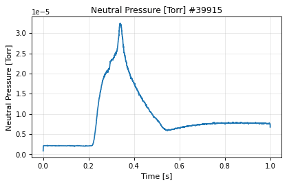
barometry_time_pressure · shot 39915 Stalebarometry_time_pressure
time
source
barometry / time / pressure · domain barometry · view model LineSeries
Neutral pressure history from the barometry gauges.
Thumbnail drawn from sample shot 39915, stale: renderer or style changed.
vaft.omas.plot_barometry_time_pressure(ods)         # from data
vaft.plot.barometry_time_pressure(model)   # from a LineSeries
Show source vaft/plot/renderers/lines.py, lines 1329–1351
@renderer(
    domain="barometry",
    subject="barometry",
    view="time",
    quantity="pressure",
    model=LineSeries,
    description="Neutral pressure history from the barometry gauges.",
    ids=("barometry",),
    required_paths=(
        "barometry.gauge.{i}.pressure.time",
        "barometry.gauge.{i}.pressure.data",
    ),
    optional_paths=("barometry.gauge.{i}.name",),
)
def barometry_time_pressure(
    model: LineSeries,
    *,
    ax: Axes | None = None,
    show: bool = False,
    **style: Any,
) -> tuple[Figure, Axes]:
    """Neutral pressure history from the barometry gauges."""
return render_line_series(model, ax=ax, show=show, **style)| IDS | barometry |
|---|---|
| Required paths | barometry.gauge.{i}.pressure.timebarometry.gauge.{i}.pressure.data |
| Optional paths | barometry.gauge.{i}.name |
| Backends | matplotlib, plotly |
| Renderer | vaft.plot.renderers.lines.barometry_time_pressure |
rogowski_coil [rogowski]
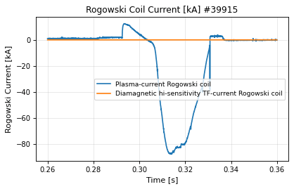
rogowski_coil_time_current · shot 39915 Stalerogowski_coil_time_current
time
source
rogowski_coil / time / current · domain magnetics · view model LineSeries
Current measured by each Rogowski coil.
Thumbnail drawn from sample shot 39915, stale: renderer or style changed.
vaft.omas.plot_rogowski_coil_time_current(ods)         # from data
vaft.plot.rogowski_coil_time_current(model)   # from a LineSeries
Show source vaft/plot/renderers/lines.py, lines 1275–1297
@renderer(
    domain="magnetics",
    subject="rogowski_coil",
    view="time",
    quantity="current",
    model=LineSeries,
    description="Current measured by each Rogowski coil.",
    ids=("magnetics",),
    required_paths=("magnetics.rogowski_coil.{i}.current.data",),
    optional_paths=(
        "magnetics.rogowski_coil.{i}.current.time",
        "magnetics.rogowski_coil.{i}.name",
    ),
)
def rogowski_coil_time_current(
    model: LineSeries,
    *,
    ax: Axes | None = None,
    show: bool = False,
    **style: Any,
) -> tuple[Figure, Axes]:
    """Current measured by each Rogowski coil."""
return render_line_series(model, ax=ax, show=show, **style)| IDS | magnetics |
|---|---|
| Required paths | magnetics.rogowski_coil.{i}.current.data |
| Optional paths | magnetics.rogowski_coil.{i}.current.timemagnetics.rogowski_coil.{i}.name |
| Backends | matplotlib, plotly |
| Renderer | vaft.plot.renderers.lines.rogowski_coil_time_current |
camera_visible
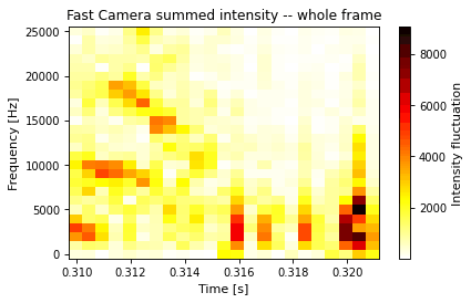
camera_visible_spectrogram · shot 40600 Stale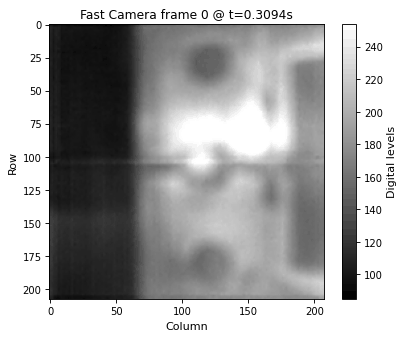
camera_visible_image · shot 40600 Stalecamera_visible_image_efit_overlaycamera_visible_image_field_line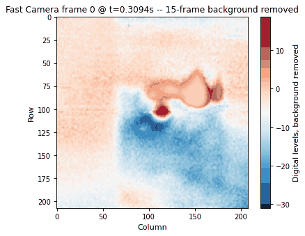
camera_visible_image_fluctuation · shot 40600 Stale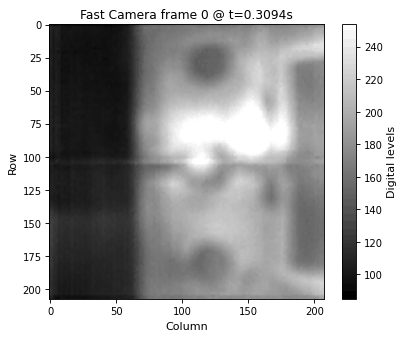
camera_visible_image_frame · shot 40600 Stale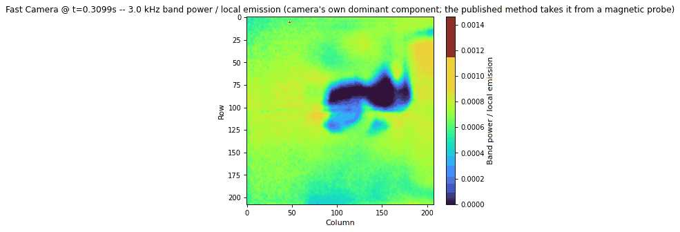
camera_visible_image_mhd_power · shot 40600 Stalecamera_visible_image_vacuum_field_line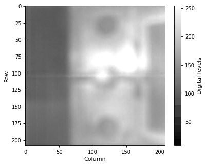
camera_visible_animation_frames · shot 40600 Stalecamera_visible_spectrogram
spectrogram
source
camera_visible / spectrogram · domain camera_visible · view model Spectrogram
Time-frequency map of the FAST-camera intensity summed over one image region, the camera side of the published camera/magnetics comparison (issue #161).
Thumbnail drawn from sample shot 40600, stale: renderer or style changed.
vaft.omas.plot_camera_visible_spectrogram(ods)         # from data
vaft.plot.camera_visible_spectrogram(model)   # from a Spectrogram
Show source vaft/plot/renderers/spectrograms.py, lines 84–105
@renderer(
    domain="camera_visible",
    subject="camera_visible",
    view="spectrogram",
    quantity="",
    model=Spectrogram,
    description=(
        "Time-frequency map of the FAST-camera intensity summed over one image "
        "region, the camera side of the published camera/magnetics comparison "
        "(issue #161)."
    ),
    ids=("camera_visible",),
    required_paths=(
        "camera_visible.channel.{i}.detector.{j}.frame.{k}.image_raw",
        "camera_visible.channel.{i}.detector.{j}.frame.{k}.time",
    ),
)
def camera_visible_spectrogram(
    model: Spectrogram, *, ax: Axes | None = None, show: bool = False, **style: Any
) -> tuple[Figure, Axes]:
    """Time-frequency map of the summed FAST-camera intensity."""
return render_spectrogram(model, ax=ax, show=show, **style)| IDS | camera_visible |
|---|---|
| Required paths | camera_visible.channel.{i}.detector.{j}.frame.{k}.image_rawcamera_visible.channel.{i}.detector.{j}.frame.{k}.time |
| Backends | matplotlib, plotly |
| Renderer | vaft.plot.renderers.spectrograms.camera_visible_spectrogram |
camera_visible_image
image
source
camera_visible / image · domain camera_visible · view model Image2D
One camera frame with optional overlays – wall, equilibrium, field line – through one projection (issue #261).
Thumbnail drawn from sample shot 40600, stale: renderer or style changed.
vaft.omas.plot_camera_visible_image(ods)         # from data
vaft.plot.camera_visible_image(model)   # from a Image2D
Show source vaft/plot/renderers/images.py, lines 182–199
@_image_renderer(
    domain="camera_visible", quantity="",
    subject="camera_visible",
    description=(
        "One camera frame with optional overlays -- wall, equilibrium, field "
        "line -- through one projection (issue #261)."
    ),
    ids=("camera_visible",),
    required_paths=(
        "camera_visible.channel.{i}.detector.{j}.frame.{k}.image_raw",
        "camera_visible.channel.{i}.detector.{j}.frame.{k}.time",
    ),
)
def camera_visible_image(
    model: Image2D, *, ax: Axes | None = None, show: bool = False, **style: Any
) -> tuple[Figure, Axes]:
    """Camera frame with optional overlays; the ``_frame``/``_efit_overlay``/``_field_line`` renderers are its presets."""
return render_image_2d(model, ax=ax, show=show, **style)| IDS | camera_visible |
|---|---|
| Required paths | camera_visible.channel.{i}.detector.{j}.frame.{k}.image_rawcamera_visible.channel.{i}.detector.{j}.frame.{k}.time |
| Backends | matplotlib |
| Renderer | vaft.plot.renderers.images.camera_visible_image |
camera_visible_image_efit_overlay
image
source
camera_visible / image / efit_overlay · domain camera_visible · view model Image2D
FAST-camera frame with the calibrated pinhole projection of the wall, LCFS, magnetic axis, and flux surfaces overlaid.
No thumbnail: no packaged sample carries the data this plot needs.
vaft.omas.plot_camera_visible_image_efit_overlay(ods)         # from data
vaft.plot.camera_visible_image_efit_overlay(model)   # from a Image2D
Show source vaft/plot/renderers/images.py, lines 261–279
@_image_renderer(
    domain="camera_visible", quantity="efit_overlay",
    subject="camera_visible",
    description=(
        "FAST-camera frame with the calibrated pinhole projection of the "
        "wall, LCFS, magnetic axis, and flux surfaces overlaid."
    ),
    ids=("camera_visible", "equilibrium", "wall"),
    required_paths=(
        "camera_visible.channel.{i}.detector.{j}.frame.{k}.image_raw",
        "equilibrium.time_slice.{i}.boundary.outline.r",
        "wall.description_2d.{i}.limiter.unit.{j}.outline.r",
    ),
)
def camera_visible_image_efit_overlay(
    model: Image2D, *, ax: Axes | None = None, show: bool = False, **style: Any
) -> tuple[Figure, Axes]:
    """FAST-camera frame with the projected EFIT/wall overlay."""
return render_image_2d(model, ax=ax, show=show, **style)| IDS | camera_visible, equilibrium, wall |
|---|---|
| Required paths | camera_visible.channel.{i}.detector.{j}.frame.{k}.image_rawequilibrium.time_slice.{i}.boundary.outline.rwall.description_2d.{i}.limiter.unit.{j}.outline.r |
| Backends | matplotlib |
| Renderer | vaft.plot.renderers.images.camera_visible_image_efit_overlay |
camera_visible_image_field_line
image
source
camera_visible / image / field_line · domain camera_visible · view model Image2D
FAST-camera frame with a traced magnetic field line projected onto it.
No thumbnail: no packaged sample carries the data this plot needs.
vaft.omas.plot_camera_visible_image_field_line(ods)         # from data
vaft.plot.camera_visible_image_field_line(model)   # from a Image2D
Show source vaft/plot/renderers/images.py, lines 282–298
@_image_renderer(
    domain="camera_visible", quantity="field_line",
    subject="camera_visible",
    description=(
        "FAST-camera frame with a traced magnetic field line projected onto it."
    ),
    ids=("camera_visible", "equilibrium"),
    required_paths=(
        "camera_visible.channel.{i}.detector.{j}.frame.{k}.image_raw",
        "equilibrium.time_slice.{i}.profiles_2d.{j}.psi",
    ),
)
def camera_visible_image_field_line(
    model: Image2D, *, ax: Axes | None = None, show: bool = False, **style: Any
) -> tuple[Figure, Axes]:
    """FAST-camera frame with a projected traced field line."""
return render_image_2d(model, ax=ax, show=show, **style)| IDS | camera_visible, equilibrium |
|---|---|
| Required paths | camera_visible.channel.{i}.detector.{j}.frame.{k}.image_rawequilibrium.time_slice.{i}.profiles_2d.{j}.psi |
| Backends | matplotlib |
| Renderer | vaft.plot.renderers.images.camera_visible_image_field_line |
camera_visible_image_fluctuation
image
source
camera_visible / image / fluctuation · domain camera_visible · view model Image2D
One FAST-camera frame with its local temporal background removed, the published step that brings fast filamentary structure out of the slowly varying line emission (issue #161).
Thumbnail drawn from sample shot 40600, stale: renderer or style changed.
vaft.omas.plot_camera_visible_image_fluctuation(ods)         # from data
vaft.plot.camera_visible_image_fluctuation(model)   # from a Image2D
Show source vaft/plot/renderers/images.py, lines 202–220
@_image_renderer(
    domain="camera_visible", quantity="fluctuation",
    subject="camera_visible",
    description=(
        "One FAST-camera frame with its local temporal background removed, the "
        "published step that brings fast filamentary structure out of the slowly "
        "varying line emission (issue #161)."
    ),
    ids=("camera_visible",),
    required_paths=(
        "camera_visible.channel.{i}.detector.{j}.frame.{k}.image_raw",
        "camera_visible.channel.{i}.detector.{j}.frame.{k}.time",
    ),
)
def camera_visible_image_fluctuation(
    model: Image2D, *, ax: Axes | None = None, show: bool = False, **style: Any
) -> tuple[Figure, Axes]:
    """FAST-camera frame with its local temporal background subtracted."""
return render_image_2d(model, ax=ax, show=show, **style)| IDS | camera_visible |
|---|---|
| Required paths | camera_visible.channel.{i}.detector.{j}.frame.{k}.image_rawcamera_visible.channel.{i}.detector.{j}.frame.{k}.time |
| Backends | matplotlib |
| Renderer | vaft.plot.renderers.images.camera_visible_image_fluctuation |
camera_visible_image_frame
image
source
camera_visible / image / frame · domain camera_visible · view model Image2D
One FAST-camera frame (raw digital levels, uncalibrated).
Thumbnail drawn from sample shot 40600, stale: renderer or style changed.
vaft.omas.plot_camera_visible_image_frame(ods)         # from data
vaft.plot.camera_visible_image_frame(model)   # from a Image2D
Show source vaft/plot/renderers/images.py, lines 244–258
@_image_renderer(
    domain="camera_visible", quantity="frame",
    subject="camera_visible",
    description="One FAST-camera frame (raw digital levels, uncalibrated).",
    ids=("camera_visible",),
    required_paths=(
        "camera_visible.channel.{i}.detector.{j}.frame.{k}.image_raw",
        "camera_visible.channel.{i}.detector.{j}.frame.{k}.time",
    ),
)
def camera_visible_image_frame(
    model: Image2D, *, ax: Axes | None = None, show: bool = False, **style: Any
) -> tuple[Figure, Axes]:
    """One FAST-camera frame (raw digital levels, uncalibrated)."""
return render_image_2d(model, ax=ax, show=show, **style)| IDS | camera_visible |
|---|---|
| Required paths | camera_visible.channel.{i}.detector.{j}.frame.{k}.image_rawcamera_visible.channel.{i}.detector.{j}.frame.{k}.time |
| Backends | matplotlib |
| Renderer | vaft.plot.renderers.images.camera_visible_image_frame |
camera_visible_image_mhd_power
image
source
camera_visible / image / mhd_power · domain camera_visible · view model Image2D
Per-pixel MHD-band power divided by the local average emission: the published spectrally filtered image, which is a band magnitude and not an inverse-transform reconstruction (issue #161).
Thumbnail drawn from sample shot 40600, stale: renderer or style changed.
vaft.omas.plot_camera_visible_image_mhd_power(ods)         # from data
vaft.plot.camera_visible_image_mhd_power(model)   # from a Image2D
Show source vaft/plot/renderers/images.py, lines 223–241
@_image_renderer(
    domain="camera_visible", quantity="mhd_power",
    subject="camera_visible",
    description=(
        "Per-pixel MHD-band power divided by the local average emission: the "
        "published spectrally filtered image, which is a band magnitude and not "
        "an inverse-transform reconstruction (issue #161)."
    ),
    ids=("camera_visible",),
    required_paths=(
        "camera_visible.channel.{i}.detector.{j}.frame.{k}.image_raw",
        "camera_visible.channel.{i}.detector.{j}.frame.{k}.time",
    ),
)
def camera_visible_image_mhd_power(
    model: Image2D, *, ax: Axes | None = None, show: bool = False, **style: Any
) -> tuple[Figure, Axes]:
    """Normalised MHD-band power of every pixel at one time."""
return render_image_2d(model, ax=ax, show=show, **style)| IDS | camera_visible |
|---|---|
| Required paths | camera_visible.channel.{i}.detector.{j}.frame.{k}.image_rawcamera_visible.channel.{i}.detector.{j}.frame.{k}.time |
| Backends | matplotlib |
| Renderer | vaft.plot.renderers.images.camera_visible_image_mhd_power |
camera_visible_image_vacuum_field_line
image
source
camera_visible / image / vacuum_field_line · domain camera_visible · view model Image2D
FAST-camera frame with vacuum field lines – coils and vessel only, never an equilibrium – traced from (R, Z) seeds at the frame's time (seeds=, ec_frequency_Hz= adds the ECR radius).
No thumbnail: shot 40600: ValueError: no calibrated camera projection is available for shot 40600: No calibrated FAST-camera pose is packaged for shot 40600. Calibrated shots: (34764, 39915, 47518). Provide pose_path to use an external pose file..
vaft.omas.plot_camera_visible_image_vacuum_field_line(ods)         # from data
vaft.plot.camera_visible_image_vacuum_field_line(model)   # from a Image2D
Show source vaft/plot/renderers/images.py, lines 301–320
@_image_renderer(
    domain="camera_visible", quantity="vacuum_field_line",
    subject="camera_visible",
    description=(
        "FAST-camera frame with vacuum field lines -- coils and vessel only, never an "
        "equilibrium -- traced from (R, Z) seeds at the frame's time (seeds=, "
        "ec_frequency_Hz= adds the ECR radius)."
    ),
    ids=("camera_visible", "pf_active", "pf_passive", "wall", "tf", "equilibrium"),
    required_paths=(
        "camera_visible.channel.{i}.detector.{j}.frame.{k}.image_raw",
        "pf_active.coil.{i}.current.data",
        "tf.b_field_tor_vacuum_r.data",
    ),
)
def camera_visible_image_vacuum_field_line(
    model: Image2D, *, ax: Axes | None = None, show: bool = False, **style: Any
) -> tuple[Figure, Axes]:
    """FAST-camera frame with projected vacuum field lines."""
return render_image_2d(model, ax=ax, show=show, **style)| IDS | camera_visible, pf_active, pf_passive, wall, tf, equilibrium |
|---|---|
| Required paths | camera_visible.channel.{i}.detector.{j}.frame.{k}.image_rawpf_active.coil.{i}.current.datatf.b_field_tor_vacuum_r.data |
| Backends | matplotlib |
| Renderer | vaft.plot.renderers.images.camera_visible_image_vacuum_field_line |
camera_visible_animation_frames
animation
source
camera_visible / animation / frames · domain camera_visible · view model ImageSequence
Animate a sequence of FAST-camera frames on a shared color scale.
Thumbnail drawn from sample shot 40600, stale: renderer or style changed.
vaft.omas.plot_camera_visible_animation_frames(ods)         # from data
vaft.plot.camera_visible_animation_frames(model)   # from a ImageSequence
Show source vaft/plot/renderers/images.py, lines 323–337
@renderer(
    domain="camera_visible", view="animation", quantity="frames", model=ImageSequence,
    subject="camera_visible",
    description="Animate a sequence of FAST-camera frames on a shared color scale.",
    ids=("camera_visible",),
    required_paths=(
        "camera_visible.channel.{i}.detector.{j}.frame.{k}.image_raw",
        "camera_visible.channel.{i}.detector.{j}.frame.{k}.time",
    ),
)
def camera_visible_animation_frames(
    model: ImageSequence, *, ax: Axes | None = None, show: bool = False, **style: Any
):
    """Animate a sequence of FAST-camera frames on a shared color scale."""
return render_image_sequence(model, ax=ax, show=show, **style)| IDS | camera_visible |
|---|---|
| Required paths | camera_visible.channel.{i}.detector.{j}.frame.{k}.image_rawcamera_visible.channel.{i}.detector.{j}.frame.{k}.time |
| Backends | matplotlib |
| Renderer | vaft.plot.renderers.images.camera_visible_animation_frames |
magnetics
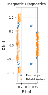
magnetics_geometry_poloidal · shot 39915 Stale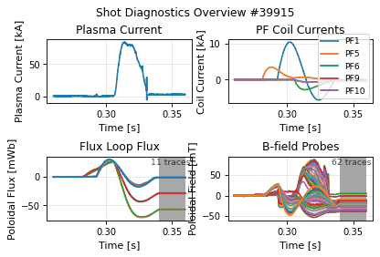
magnetics_overview · shot 39915 Stale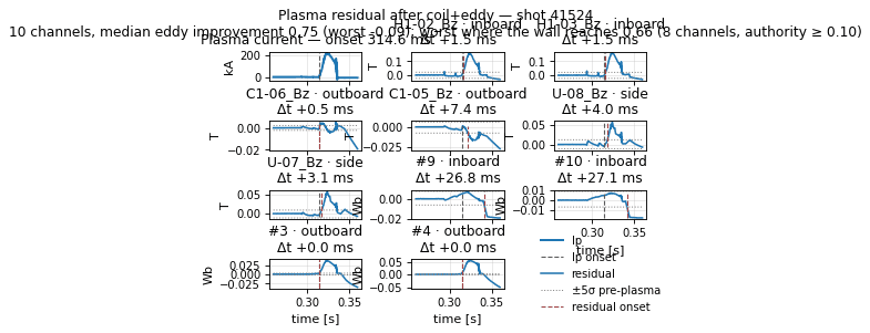
magnetics_overview_plasma_residual · shot 41524 Stale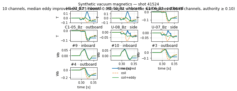
magnetics_overview_vacuum · shot 41524 Stale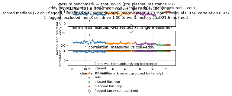
magnetics_overview_vacuum_benchmark · shot 39915 Stalemagnetics_table_vacuum_benchmarkmagnetics_table_vacuum_benchmark_aggregatemagnetics_geometry_poloidal
geometry
source
magnetics / geometry / poloidal · domain magnetics · view model GeometryLayers
Flux-loop and B-field-probe positions in the poloidal plane.
Thumbnail drawn from sample shot 39915, stale: renderer or style changed.
vaft.omas.plot_magnetics_geometry_poloidal(ods)         # from data
vaft.plot.magnetics_geometry_poloidal(model)   # from a GeometryLayers
Show source vaft/plot/renderers/geometry.py, lines 312–327
@_geometry_renderer(
    domain="magnetics", quantity="poloidal",
    subject="magnetics",
    description="Flux-loop and B-field-probe positions in the poloidal plane.",
    ids=("magnetics",),
    required_paths=(),
    optional_paths=("magnetics.flux_loop.{i}.position.0.r",
                    "magnetics.flux_loop.{i}.position.0.z",
                    "magnetics.b_field_pol_probe.{i}.position.r",
                    "magnetics.b_field_pol_probe.{i}.position.z"),
)
def magnetics_geometry_poloidal(
    model: GeometryLayers, *, ax: Axes | None = None, show: bool = False, **style: Any
) -> tuple[Figure, Axes]:
    """Flux-loop and B-field-probe positions in the poloidal plane."""
return render_geometry_layers(model, ax=ax, show=show, **style)| IDS | magnetics |
|---|---|
| Required paths | — |
| Optional paths | magnetics.flux_loop.{i}.position.0.rmagnetics.flux_loop.{i}.position.0.zmagnetics.b_field_pol_probe.{i}.position.rmagnetics.b_field_pol_probe.{i}.position.z |
| Backends | matplotlib |
| Renderer | vaft.plot.renderers.geometry.magnetics_geometry_poloidal |
magnetics_overview
overview
source
magnetics / overview / diagnostics · domain magnetics · view model Panels
Shot diagnostic overview: current, field, flux and geometry panels.
Thumbnail drawn from sample shot 39915, stale: renderer or style changed.
vaft.omas.plot_magnetics_overview(ods)         # from data
vaft.plot.magnetics_overview(model)   # from a Panels
Show source vaft/plot/renderers/panels.py, lines 1206–1219
@_panel_renderer(
    domain="magnetics",
    subject="magnetics",
    view="overview",
    quantity="diagnostics",
    description="Shot diagnostic overview: current, field, flux and geometry panels.",
    ids=("magnetics", "pf_active", "tf", "equilibrium"),
    required_paths=("magnetics.ip.0.data",),
)
def magnetics_overview(
    model: Panels, *, ax: Any = None, show: bool = False, **style: Any
) -> tuple[Figure, np.ndarray]:
    """Shot diagnostic overview panels."""
return render_panels(model, ax=ax, show=show, **style)| IDS | magnetics, pf_active, tf, equilibrium |
|---|---|
| Required paths | magnetics.ip.0.data |
| Backends | matplotlib, plotly |
| Renderer | vaft.plot.renderers.panels.magnetics_overview |
magnetics_overview_plasma_residual
overview
source
magnetics / overview / plasma_residual · domain magnetics · view model Panels
Residual of measured minus coil+eddy synthetic magnetics against the pre-plasma noise band, with the plasma-current and residual onsets.
Thumbnail drawn from sample shot 41524, stale: renderer or style changed.
vaft.omas.plot_magnetics_overview_plasma_residual(ods)         # from data
vaft.plot.magnetics_overview_plasma_residual(model)   # from a Panels
Show source vaft/plot/renderers/panels.py, lines 1315–1332
@_panel_renderer(
    domain="magnetics",
    subject="magnetics",
    view="overview",
    quantity="plasma_residual",
    description=(
        "Residual of measured minus coil+eddy synthetic magnetics against the "
        "pre-plasma noise band, with the plasma-current and residual onsets."
    ),
    ids=_VACUUM_IDS,
    required_paths=_VACUUM_REQUIRED + ("magnetics.ip.{i}.data",),
    optional_paths=_VACUUM_OPTIONAL,
)
def magnetics_overview_plasma_residual(
    model: Panels, *, ax: Any = None, show: bool = False, **style: Any
) -> tuple[Figure, np.ndarray]:
    """Plasma-signal residual left by the coil+eddy synthetic vacuum response."""
return render_panels(model, ax=ax, show=show, **style)| IDS | magnetics, pf_active, pf_passive |
|---|---|
| Required paths | pf_active.coil.{i}.current.datapf_passive.loop.{i}.currentmagnetics.ip.{i}.data |
| Optional paths | magnetics.b_field_pol_probe.{i}.field.datamagnetics.flux_loop.{i}.flux.data |
| Backends | matplotlib, plotly |
| Renderer | vaft.plot.renderers.panels.magnetics_overview_plasma_residual |
magnetics_overview_vacuum
overview
source
magnetics / overview / vacuum · domain magnetics · view model Panels
Measured, coil-only and coil+eddy synthetic magnetics per channel: the forward-modeled validation of an eddy-current reconstruction.
Thumbnail drawn from sample shot 41524, stale: renderer or style changed.
vaft.omas.plot_magnetics_overview_vacuum(ods)         # from data
vaft.plot.magnetics_overview_vacuum(model)   # from a Panels
Show source vaft/plot/renderers/panels.py, lines 1295–1312
@_panel_renderer(
    domain="magnetics",
    subject="magnetics",
    view="overview",
    quantity="vacuum",
    description=(
        "Measured, coil-only and coil+eddy synthetic magnetics per channel: "
        "the forward-modeled validation of an eddy-current reconstruction."
    ),
    ids=_VACUUM_IDS,
    required_paths=_VACUUM_REQUIRED,
    optional_paths=_VACUUM_OPTIONAL,
)
def magnetics_overview_vacuum(
    model: Panels, *, ax: Any = None, show: bool = False, **style: Any
) -> tuple[Figure, np.ndarray]:
    """Measured against coil-only and coil+eddy synthetic vacuum magnetics."""
return render_panels(model, ax=ax, show=show, **style)| IDS | magnetics, pf_active, pf_passive |
|---|---|
| Required paths | pf_active.coil.{i}.current.datapf_passive.loop.{i}.current |
| Optional paths | magnetics.b_field_pol_probe.{i}.field.datamagnetics.flux_loop.{i}.flux.data |
| Backends | matplotlib, plotly |
| Renderer | vaft.plot.renderers.panels.magnetics_overview_vacuum |
magnetics_overview_vacuum_benchmark
overview
source
magnetics / overview / vacuum_benchmark · domain magnetics · view model Panels
Per-channel scores of the plasma-free vacuum benchmark (issue #190): eddy improvement against a zero reference, normalized residual and correlation, channels grouped and coloured by family, flagged probes hollow.
Interpretation
The shot is run through vaft.validation.vacuum_benchmark.run_benchmark_case
– the passive wall re-solved from the measured PF currents alone over the
plasma-free stretch – and each scored B probe and flux loop is one point
per panel, at its position in the benchmark’s order (the # column of
magnetics_table_vacuum_benchmark), coloured by family. The top
panel is the eddy improvement 1 - RMS(measured - (coil+eddy)) /
RMS(measured - coil), what the wall model is worth on that channel, with
a dashed line at zero where the wall term adds nothing; the middle panel the residual RMS as a fraction of the
channel’s swing; the bottom the correlation of measured with coil+eddy,
which near 1 beside a large residual points at a gain rather than at the
wall. Read together they show which families and which individual
channels the vacuum model reproduces and where it falls away. A probe
the benchmark flags as contradicting its own array is drawn hollow and
named in the legend: scored, but a sensor finding kept out of the scored
medians. Excluded channels (too few usable samples) are not drawn; the
title names them, with the window, coil drive and solver history the case
was measured under.
Limitations
The zero line is a reference, not a threshold: the benchmark states no acceptance bound and no verdict, and neither colour nor marker grades a channel. The horizontal axis is a channel index, not a geometry; the table gives each index its channel name. Scores from one shot’s plasma-free stretch say nothing about the model with plasma, and a low improvement where the eddy term is a small share of the reading (the table’s wall authority) is a rounding of the model’s error, not a finding about the wall.
See Also
See Also
magnetics_table_vacuum_benchmark : the same scores with channel names and reasons. magnetics_table_vacuum_benchmark_aggregate : the benchmark across shots. magnetics_overview_vacuum : the measured, coil and coil+eddy waveforms behind the scores.
Thumbnail drawn from sample shot 39915, stale: renderer or style changed.
vaft.omas.plot_magnetics_overview_vacuum_benchmark(ods)         # from data
vaft.plot.magnetics_overview_vacuum_benchmark(model)   # from a Panels
Show source vaft/plot/renderers/panels.py, lines 1335–1408
@_panel_renderer(
    domain="magnetics",
    subject="magnetics",
    view="overview",
    quantity="vacuum_benchmark",
    description=(
        "Per-channel scores of the plasma-free vacuum benchmark (issue #190): eddy "
        "improvement against a zero reference, normalized residual and correlation, "
        "channels grouped and coloured by family, flagged probes hollow."
    ),
    # Every root the builder reads (recipes._VACUUM_BENCHMARK_ROOTS): the UV
    # lines and the summary cut the plasma-free interval, so a loader that
    # selects by ids must not drop them.
    ids=(
        "pf_active", "pf_passive", "magnetics", "em_coupling", "wall",
        "tf", "spectrometer_uv", "summary",
    ),
    required_paths=(
        "pf_active.time",
        "pf_active.coil.{i}.current.data",
        "pf_passive.loop.{i}.resistance",
    ),
    optional_paths=_VACUUM_OPTIONAL + ("magnetics.ip.{i}.data", "em_coupling.mutual_passive_active"),
)
def magnetics_overview_vacuum_benchmark(
    model: Panels, *, ax: Any = None, show: bool = False, **style: Any
) -> tuple[Figure, np.ndarray]:
    """The vacuum benchmark's per-channel scores of one shot, channel by channel.

    Interpretation
    --------------
    The shot is run through :func:`vaft.validation.vacuum_benchmark.run_benchmark_case`
    -- the passive wall re-solved from the measured PF currents alone over the
    plasma-free stretch -- and each scored B probe and flux loop is one point
    per panel, at its position in the benchmark's order (the ``#`` column of
    :func:`magnetics_table_vacuum_benchmark`), coloured by family.  The top
    panel is the eddy improvement 1 - RMS(measured - (coil+eddy)) /
    RMS(measured - coil), what the wall model is worth on that channel, with
    a dashed line at zero where the wall term adds nothing; the middle panel the residual RMS as a fraction of the
    channel's swing; the bottom the correlation of measured with coil+eddy,
    which near 1 beside a large residual points at a gain rather than at the
    wall.  Read together they show which families and which individual
    channels the vacuum model reproduces and where it falls away.  A probe
    the benchmark flags as contradicting its own array is drawn hollow and
    named in the legend: scored, but a sensor finding kept out of the scored
    medians.  Excluded channels (too few usable samples) are not drawn; the
    title names them, with the window, coil drive and solver history the case
    was measured under.

    Options
    -------
    ``per_family=``, ``resistance_scale=`` and ``n_tau=`` are passed to the
    benchmark as in :func:`magnetics_table_vacuum_benchmark`: the channels per
    family, one global factor on every passive-loop resistance, and the wall
    time constants of solver history before the validation window opens.

    Limitations
    -----------
    The zero line is a reference, not a threshold: the benchmark states no
    acceptance bound and no verdict, and neither colour nor marker grades a
    channel.  The horizontal axis is a channel index, not a geometry; the
    table gives each index its channel name.  Scores from one shot's
    plasma-free stretch say nothing about the model with plasma, and a low
    improvement where the eddy term is a small share of the reading (the
    table's wall authority) is a rounding of the model's error, not a finding
    about the wall.

    See Also
    --------
    magnetics_table_vacuum_benchmark : the same scores with channel names and reasons.
    magnetics_table_vacuum_benchmark_aggregate : the benchmark across shots.
    magnetics_overview_vacuum : the measured, coil and coil+eddy waveforms behind the scores.
    """
return render_panels(model, ax=ax, show=show, **style)| IDS | pf_active, pf_passive, magnetics, em_coupling, wall, tf, spectrometer_uv, summary |
|---|---|
| Required paths | pf_active.timepf_active.coil.{i}.current.datapf_passive.loop.{i}.resistance |
| Optional paths | magnetics.b_field_pol_probe.{i}.field.datamagnetics.flux_loop.{i}.flux.datamagnetics.ip.{i}.dataem_coupling.mutual_passive_active |
| Backends | matplotlib, plotly |
| Renderer | vaft.plot.renderers.panels.magnetics_overview_vacuum_benchmark |
magnetics_table_vacuum_benchmark
table
source
magnetics / table / vacuum_benchmark · domain magnetics · view model Table
The plasma-free vacuum benchmark of one shot (issue #190), one row per channel: family, kind, status (evaluated, flagged, excluded), eddy improvement, normalized residual, correlation, wall authority and the reason a channel is flagged or excluded; windows, solver history, coil drive and scored medians in the caption.
Interpretation
The shot is run through vaft.validation.vacuum_benchmark.run_benchmark_case:
the passive wall is re-solved from the measured PF currents alone over the
plasma-free stretch, and every usable B probe and flux loop is compared
with the coil-only and coil+eddy forward response inside the validation
window. One row per scored channel, in the benchmark’s order (grouped by
family): the eddy improvement 1 - RMS(measured - (coil+eddy)) /
RMS(measured - coil) – what the wall model is worth on that channel –
the residual RMS as a fraction of the
channel’s swing, the correlation of measured with coil+eddy (near 1 with a
large residual points at a gain, not the wall), and the wall authority, the
eddy term’s share of the reading in whose light a small or negative
improvement is read. Status is a fact, not a grade: flagged is a probe
that contradicts its own array, scored but kept out of the medians as a
sensor finding; excluded had too few usable samples. The caption
states the case type, the validation window inside the solver-input
window, the solver history against the slowest wall time constant, the
coil drive inside the window and the scored medians, so a row can be
traced to the conditions it was measured under. The table answers which
channels and families the wall model reproduces and which it does not.
Limitations
The benchmark states no acceptance threshold and no verdict, and neither does the table: #190 defers acceptance bounds until the VEST benchmark distribution has been inspected. A score is measured against one shot’s plasma-free stretch, so it says nothing about the model with plasma, and a low improvement where the wall authority is small is a rounding of the model’s error rather than a finding about the wall. A flagged probe is a sensor finding from its array neighbours, not a proof that the probe is faulty. A case the coils did not drive inside its window is reported (the caption says so) and its improvements are ratios of noise.
See Also
See Also
magnetics_overview_vacuum_benchmark : the same scores drawn per channel. magnetics_table_vacuum_benchmark_aggregate : the benchmark across shots. magnetics_overview_vacuum : one shot’s measured, coil and coil+eddy waveforms.
No thumbnail: a table/text view is presented as text, not drawn as a figure.
vaft.omas.plot_magnetics_table_vacuum_benchmark(ods)         # from data
vaft.plot.magnetics_table_vacuum_benchmark(model) # from a Table| IDS | pf_active, pf_passive, magnetics, em_coupling, wall, tf, spectrometer_uv, summary |
|---|---|
| Required paths | pf_active.timepf_active.coil.{i}.current.datapf_passive.loop.{i}.resistance |
| Optional paths | magnetics.b_field_pol_probe.{i}.field.datamagnetics.flux_loop.{i}.flux.datamagnetics.ip.{i}.dataem_coupling.mutual_passive_active |
| Backends | |
| Renderer | vaft.plot.renderers.tables.magnetics_table_vacuum_benchmark |
magnetics_table_vacuum_benchmark_aggregate
table
source
magnetics / table / vacuum_benchmark_aggregate · domain magnetics · view model Table
The plasma-free vacuum benchmark across shots (issue #190): median eddy improvement, normalized residual and correlation and the worst channel by case, family, PF excitation and machine era; undriven cases, flagged channels and the summary in the caption.
Interpretation
Every entry is run through vaft.validation.vacuum_benchmark.run_benchmark_case
and the cases are cross-tabulated by
vaft.validation.vacuum_benchmark.aggregate_benchmark. One row per
group of each axis – case (the entry’s label), magnetic family, PF
excitation (the coils that carried current) and machine era (the VEST era
the pulse falls in, unknown without a pulse) – with the number of cases
and channels in it, the median eddy improvement, normalized residual and
correlation, and the channel with the lowest improvement. Which axis a poor
median concentrates on is the diagnosis the cross-tabs exist for: one
channel across excitations points at probe calibration or geometry, many
channels whenever one PF coil dominates at that coil, a change across eras
at the static model’s provenance, one shot among consistent neighbours at
that shot’s acquisition. An entry that cannot supply a plasma-free case
– it lacks the PF or passive-loop circuits the case is solved from, it
has no usable magnetic channel or no em_coupling, or the benchmark
refuses it – is a case row with the reason, never dropped, and so is a
case whose every channel was excluded. The caption lists the cases the
coils did not drive, the flagged probes per case and the summary medians
over driven, unflagged channel rows.
Limitations
No threshold and no verdict, as in the benchmark itself. The cross-tab medians count every evaluated channel, the flagged and undriven ones too (the notes say so); only the caption’s summary leaves them out. A median over a group of one case is that case, not a distribution, and the packaged samples are few: a cross-tab over them shows the structure of the analysis, not the VEST benchmark distribution.
See Also
See Also
magnetics_table_vacuum_benchmark : one case, channel by channel. magnetics_overview_vacuum_benchmark : one case’s scores drawn per channel.
No thumbnail: a table/text view is presented as text, not drawn as a figure.
vaft.omas.plot_magnetics_table_vacuum_benchmark_aggregate(ods)         # from data
vaft.plot.magnetics_table_vacuum_benchmark_aggregate(model)   # from a Table
Show source vaft/plot/renderers/tables.py, lines 840–913
@renderer(
    domain="magnetics",
    subject="magnetics",
    view="table",
    quantity="vacuum_benchmark_aggregate",
    model=Table,
    description=(
        "The plasma-free vacuum benchmark across shots (issue #190): median eddy "
        "improvement, normalized residual and correlation and the worst channel by case, "
        "family, PF excitation and machine era; undriven cases, flagged channels and the "
        "summary in the caption."
    ),
    ids=_BENCHMARK_IDS,
    required_paths=_BENCHMARK_REQUIRED,
    optional_paths=_BENCHMARK_OPTIONAL,
)
def magnetics_table_vacuum_benchmark_aggregate(model: Table, *, show: bool = False) -> RenderedTable:
    """The vacuum benchmark across shots, by case, family, excitation and machine era.

    Parameters
    ----------
    model : Table
        The table the adapter built.
    show : bool
        Print the text form.

    Returns
    -------
    RenderedTable
        Text, Markdown and HTML renderings of the table.

    Interpretation
    --------------
    Every entry is run through :func:`vaft.validation.vacuum_benchmark.run_benchmark_case`
    and the cases are cross-tabulated by
    :func:`vaft.validation.vacuum_benchmark.aggregate_benchmark`.  One row per
    group of each axis -- case (the entry's label), magnetic family, PF
    excitation (the coils that carried current) and machine era (the VEST era
    the pulse falls in, ``unknown`` without a pulse) -- with the number of cases
    and channels in it, the median eddy improvement, normalized residual and
    correlation, and the channel with the lowest improvement.  Which axis a poor
    median concentrates on is the diagnosis the cross-tabs exist for: one
    channel across excitations points at probe calibration or geometry, many
    channels whenever one PF coil dominates at that coil, a change across eras
    at the static model's provenance, one shot among consistent neighbours at
    that shot's acquisition.  An entry that cannot supply a plasma-free case
    -- it lacks the PF or passive-loop circuits the case is solved from, it
    has no usable magnetic channel or no ``em_coupling``, or the benchmark
    refuses it -- is a case row with the reason, never dropped, and so is a
    case whose every channel was excluded.  The caption lists the cases the
    coils did not drive, the flagged probes per case and the summary medians
    over driven, unflagged channel rows.

    Options
    -------
    ``per_family=``, ``resistance_scale=`` and ``n_tau=`` are passed to every
    case as in :func:`magnetics_table_vacuum_benchmark`; ``label=`` names the
    entries, and so the case rows.  ``title=`` replaces the title.

    Limitations
    -----------
    No threshold and no verdict, as in the benchmark itself.  The cross-tab
    medians count every evaluated channel, the flagged and undriven ones too
    (the notes say so); only the caption's summary leaves them out.  A median
    over a group of one case is that case, not a distribution, and the
    packaged samples are few: a cross-tab over them shows the structure of the
    analysis, not the VEST benchmark distribution.

    See Also
    --------
    magnetics_table_vacuum_benchmark : one case, channel by channel.
    magnetics_overview_vacuum_benchmark : one case's scores drawn per channel.
    """
return render_table(model, show=show)| IDS | pf_active, pf_passive, magnetics, em_coupling, wall, tf, spectrometer_uv, summary |
|---|---|
| Required paths | pf_active.timepf_active.coil.{i}.current.datapf_passive.loop.{i}.resistance |
| Optional paths | magnetics.b_field_pol_probe.{i}.field.datamagnetics.flux_loop.{i}.flux.datamagnetics.ip.{i}.dataem_coupling.mutual_passive_active |
| Backends | |
| Renderer | vaft.plot.renderers.tables.magnetics_table_vacuum_benchmark_aggregate |
Machine subjects
wall
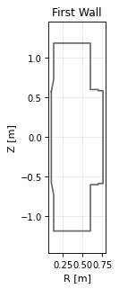
wall_geometry_poloidal · shot 39915 Stalewall_geometry_poloidal
geometry
source
wall / geometry / poloidal · domain wall · view model GeometryLayers
First-wall and limiter outline in the poloidal plane.
Thumbnail drawn from sample shot 39915, stale: renderer or style changed.
vaft.omas.plot_wall_geometry_poloidal(ods)         # from data
vaft.plot.wall_geometry_poloidal(model)   # from a GeometryLayers
Show source vaft/plot/renderers/geometry.py, lines 330–342
@_geometry_renderer(
    domain="wall", quantity="poloidal",
    subject="wall",
    description="First-wall and limiter outline in the poloidal plane.",
    ids=("wall",),
    required_paths=("wall.description_2d.{i}.limiter.unit.{j}.outline.r",
                    "wall.description_2d.{i}.limiter.unit.{j}.outline.z"),
)
def wall_geometry_poloidal(
    model: GeometryLayers, *, ax: Axes | None = None, show: bool = False, **style: Any
) -> tuple[Figure, Axes]:
    """First-wall and limiter outline in the poloidal plane."""
return render_geometry_layers(model, ax=ax, show=show, **style)| IDS | wall |
|---|---|
| Required paths | wall.description_2d.{i}.limiter.unit.{j}.outline.rwall.description_2d.{i}.limiter.unit.{j}.outline.z |
| Backends | matplotlib |
| Renderer | vaft.plot.renderers.geometry.wall_geometry_poloidal |
pf_coil [pf_active]
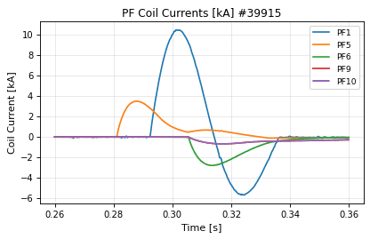
pf_coil_time_current · shot 39915 Stale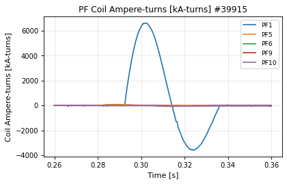
pf_coil_time_current_turns · shot 39915 Stale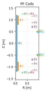
pf_coil_geometry_poloidal · shot 39915 Stalepf_coil_time_current
time
source
pf_coil / time / current · domain pf_active · view model LineSeries
Per-coil PF current history.
Thumbnail drawn from sample shot 39915, stale: renderer or style changed.
vaft.omas.plot_pf_coil_time_current(ods)         # from data
vaft.plot.pf_coil_time_current(model)   # from a LineSeries
Show source vaft/plot/renderers/lines.py, lines 558–580
@renderer(
    domain="pf_active",
    subject="pf_coil",
    view="time",
    quantity="current",
    model=LineSeries,
    description="Per-coil PF current history.",
    ids=("pf_active",),
    required_paths=(
        "pf_active.time",
        "pf_active.coil.{i}.current.data",
    ),
    optional_paths=("pf_active.coil.{i}.name",),
)
def pf_coil_time_current(
    model: LineSeries,
    *,
    ax: Axes | None = None,
    show: bool = False,
    **style: Any,
) -> tuple[Figure, Axes]:
    """Per-coil PF current history."""
return render_line_series(model, ax=ax, show=show, **style)| IDS | pf_active |
|---|---|
| Required paths | pf_active.timepf_active.coil.{i}.current.data |
| Optional paths | pf_active.coil.{i}.name |
| Backends | matplotlib, plotly |
| Renderer | vaft.plot.renderers.lines.pf_coil_time_current |
pf_coil_time_current_turns
time
source
pf_coil / time / current_turns · domain pf_active · view model LineSeries
Per-coil PF current multiplied by the signed turn count (ampere-turns).
Thumbnail drawn from sample shot 39915, stale: renderer or style changed.
vaft.omas.plot_pf_coil_time_current_turns(ods)         # from data
vaft.plot.pf_coil_time_current_turns(model)   # from a LineSeries
Show source vaft/plot/renderers/lines.py, lines 583–606
@renderer(
    domain="pf_active",
    subject="pf_coil",
    view="time",
    quantity="current_turns",
    model=LineSeries,
    description="Per-coil PF current multiplied by the signed turn count (ampere-turns).",
    ids=("pf_active",),
    required_paths=(
        "pf_active.time",
        "pf_active.coil.{i}.current.data",
        "pf_active.coil.{i}.element.{j}.turns_with_sign",
    ),
    optional_paths=("pf_active.coil.{i}.name",),
)
def pf_coil_time_current_turns(
    model: LineSeries,
    *,
    ax: Axes | None = None,
    show: bool = False,
    **style: Any,
) -> tuple[Figure, Axes]:
    """Per-coil PF current multiplied by the signed turn count (ampere-turns)."""
return render_line_series(model, ax=ax, show=show, **style)| IDS | pf_active |
|---|---|
| Required paths | pf_active.timepf_active.coil.{i}.current.datapf_active.coil.{i}.element.{j}.turns_with_sign |
| Optional paths | pf_active.coil.{i}.name |
| Backends | matplotlib, plotly |
| Renderer | vaft.plot.renderers.lines.pf_coil_time_current_turns |
pf_coil_geometry_poloidal
geometry
source
pf_coil / geometry / poloidal · domain pf_active · view model GeometryLayers
PF coil cross-sections in the poloidal plane: every element of every coil, as the rectangle or outline the IDS stores.
Thumbnail drawn from sample shot 39915, stale: renderer or style changed.
vaft.omas.plot_pf_coil_geometry_poloidal(ods)         # from data
vaft.plot.pf_coil_geometry_poloidal(model)   # from a GeometryLayers
Show source vaft/plot/renderers/geometry.py, lines 237–252
@_geometry_renderer(
    domain="pf_active", quantity="poloidal",
    subject="pf_coil",
    description="PF coil cross-sections in the poloidal plane: every element "
                "of every coil, as the rectangle or outline the IDS stores.",
    ids=("pf_active",),
    required_paths=("pf_active.coil.{i}.element.{j}.geometry.geometry_type",),
    optional_paths=("pf_active.coil.{i}.name",
                    "pf_active.coil.{i}.element.{j}.geometry.rectangle.r",
                    "pf_active.coil.{i}.element.{j}.geometry.outline.r"),
)
def pf_coil_geometry_poloidal(
    model: GeometryLayers, *, ax: Axes | None = None, show: bool = False, **style: Any
) -> tuple[Figure, Axes]:
    """PF coil outlines in the poloidal plane."""
return render_geometry_layers(model, ax=ax, show=show, **style)| IDS | pf_active |
|---|---|
| Required paths | pf_active.coil.{i}.element.{j}.geometry.geometry_type |
| Optional paths | pf_active.coil.{i}.namepf_active.coil.{i}.element.{j}.geometry.rectangle.rpf_active.coil.{i}.element.{j}.geometry.outline.r |
| Backends | matplotlib |
| Renderer | vaft.plot.renderers.geometry.pf_coil_geometry_poloidal |
tf_coil [tf]
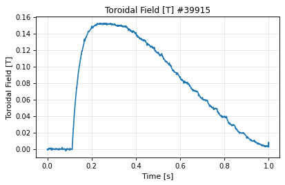
tf_coil_time_b_t · shot 39915 Stale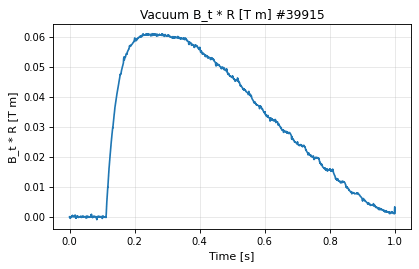
tf_coil_time_b_t_vacuum_r · shot 39915 Stale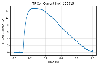
tf_coil_time_current · shot 39915 Staletf_coil_time_b_t
time
source
tf_coil / time / b_t · domain tf · view model LineSeries
Toroidal field history at the reference radius.
Thumbnail drawn from sample shot 39915, stale: renderer or style changed.
vaft.omas.plot_tf_coil_time_b_t(ods)         # from data
vaft.plot.tf_coil_time_b_t(model)   # from a LineSeries
Show source vaft/plot/renderers/lines.py, lines 1149–1171
@renderer(
    domain="tf",
    subject="tf_coil",
    view="time",
    quantity="b_t",
    model=LineSeries,
    description="Toroidal field history at the reference radius.",
    ids=("tf",),
    required_paths=(
        "tf.time",
        "tf.b_field_tor_vacuum_r.data",
    ),
    optional_paths=("tf.r0",),
)
def tf_coil_time_b_t(
    model: LineSeries,
    *,
    ax: Axes | None = None,
    show: bool = False,
    **style: Any,
) -> tuple[Figure, Axes]:
    """Toroidal field history at the reference radius."""
return render_line_series(model, ax=ax, show=show, **style)| IDS | tf |
|---|---|
| Required paths | tf.timetf.b_field_tor_vacuum_r.data |
| Optional paths | tf.r0 |
| Backends | matplotlib, plotly |
| Renderer | vaft.plot.renderers.lines.tf_coil_time_b_t |
tf_coil_time_b_t_vacuum_r
time
source
tf_coil / time / b_t_vacuum_r · domain tf · view model LineSeries
Vacuum toroidal field times major radius (B_t * R).
Thumbnail drawn from sample shot 39915, stale: renderer or style changed.
vaft.omas.plot_tf_coil_time_b_t_vacuum_r(ods)         # from data
vaft.plot.tf_coil_time_b_t_vacuum_r(model)   # from a LineSeries
Show source vaft/plot/renderers/lines.py, lines 1174–1196
@renderer(
    domain="tf",
    subject="tf_coil",
    view="time",
    quantity="b_t_vacuum_r",
    model=LineSeries,
    description="Vacuum toroidal field times major radius (B_t * R).",
    ids=("tf",),
    required_paths=(
        "tf.time",
        "tf.b_field_tor_vacuum_r.data",
    ),
    optional_paths=(),
)
def tf_coil_time_b_t_vacuum_r(
    model: LineSeries,
    *,
    ax: Axes | None = None,
    show: bool = False,
    **style: Any,
) -> tuple[Figure, Axes]:
    """Vacuum toroidal field times major radius (B_t * R)."""
return render_line_series(model, ax=ax, show=show, **style)| IDS | tf |
|---|---|
| Required paths | tf.timetf.b_field_tor_vacuum_r.data |
| Backends | matplotlib, plotly |
| Renderer | vaft.plot.renderers.lines.tf_coil_time_b_t_vacuum_r |
tf_coil_time_current
time
source
tf_coil / time / current · domain tf · view model LineSeries
TF coil current history.
Thumbnail drawn from sample shot 39915, stale: renderer or style changed.
vaft.omas.plot_tf_coil_time_current(ods)         # from data
vaft.plot.tf_coil_time_current(model)   # from a LineSeries
Show source vaft/plot/renderers/lines.py, lines 1199–1221
@renderer(
    domain="tf",
    subject="tf_coil",
    view="time",
    quantity="current",
    model=LineSeries,
    description="TF coil current history.",
    ids=("tf",),
    required_paths=(
        "tf.time",
        "tf.coil.{i}.current.data",
    ),
    optional_paths=("tf.coil.{i}.name",),
)
def tf_coil_time_current(
    model: LineSeries,
    *,
    ax: Axes | None = None,
    show: bool = False,
    **style: Any,
) -> tuple[Figure, Axes]:
    """TF coil current history."""
return render_line_series(model, ax=ax, show=show, **style)| IDS | tf |
|---|---|
| Required paths | tf.timetf.coil.{i}.current.data |
| Optional paths | tf.coil.{i}.name |
| Backends | matplotlib, plotly |
| Renderer | vaft.plot.renderers.lines.tf_coil_time_current |
passive_structure [pf_passive]
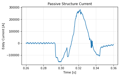
passive_structure_time_current · shot 41524 Stale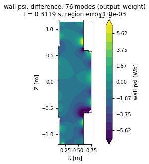
passive_structure_field_wall_reduction · shot 39915 Stale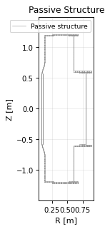
passive_structure_geometry_poloidal · shot 39915 Stale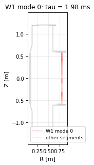
passive_structure_geometry_wall_mode · shot 39915 Stale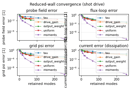
passive_structure_overview_wall_reduction · shot 39915 Stale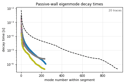
passive_structure_overview_wall_time · shot 39915 Stalepassive_structure_time_current
time
source
passive_structure / time / current · domain pf_passive · view model LineSeries
Eddy current induced in the passive structure, summed over loops.
Thumbnail drawn from sample shot 41524, stale: renderer or style changed.
vaft.omas.plot_passive_structure_time_current(ods)         # from data
vaft.plot.passive_structure_time_current(model)   # from a LineSeries
Show source vaft/plot/renderers/lines.py, lines 533–555
@renderer(
    domain="pf_passive",
    subject="passive_structure",
    view="time",
    quantity="current",
    model=LineSeries,
    description="Eddy current induced in the passive structure, summed over loops.",
    ids=("pf_passive",),
    required_paths=(
        "pf_passive.time",
        "pf_passive.loop.{i}.current",
    ),
    optional_paths=("pf_passive.loop.{i}.name",),
)
def passive_structure_time_current(
    model: LineSeries,
    *,
    ax: Axes | None = None,
    show: bool = False,
    **style: Any,
) -> tuple[Figure, Axes]:
    """Eddy current in the passive structure."""
return render_line_series(model, ax=ax, show=show, **style)| IDS | pf_passive |
|---|---|
| Required paths | pf_passive.timepf_passive.loop.{i}.current |
| Optional paths | pf_passive.loop.{i}.name |
| Backends | matplotlib, plotly |
| Renderer | vaft.plot.renderers.lines.passive_structure_time_current |
passive_structure_field_wall_reduction
field
source
passive_structure / field / wall_reduction · domain machine · view model Field2D
The passive wall's poloidal flux on the equilibrium region – full, reduced, or their difference – at one instant of the shot's PF programme (vaft #494, vfit #10).
Thumbnail drawn from sample shot 39915, stale: renderer or style changed.
vaft.omas.plot_passive_structure_field_wall_reduction(ods)         # from data
vaft.plot.passive_structure_field_wall_reduction(model)   # from a Field2D
Show source vaft/plot/renderers/fields.py, lines 337–354
@_field_renderer(
    domain="machine", quantity="wall_reduction",
    subject="passive_structure",
    description="The passive wall's poloidal flux on the equilibrium region -- "
                "full, reduced, or their difference -- at one instant of the "
                "shot's PF programme (vaft #494, vfit #10).",
    ids=("pf_active", "pf_passive", "em_coupling", "wall"),
    required_paths=("pf_passive.loop.{i}.resistance",
                    "pf_active.coil.{i}.element.{j}.geometry.geometry_type",
                    "pf_active.coil.{i}.current.data",
                    "wall.description_2d.{i}.limiter.unit.{j}.outline.r"),
    optional_paths=("em_coupling.mutual_passive_passive",),
)
def passive_structure_field_wall_reduction(
    model: Field2D, *, ax: Axes | None = None, show: bool = False, **style: Any
) -> tuple[Figure, Axes]:
    """Full, reduced or difference wall flux map on the equilibrium region."""
return render_field_2d(model, ax=ax, show=show, **style)| IDS | pf_active, pf_passive, em_coupling, wall |
|---|---|
| Required paths | pf_passive.loop.{i}.resistancepf_active.coil.{i}.element.{j}.geometry.geometry_typepf_active.coil.{i}.current.datawall.description_2d.{i}.limiter.unit.{j}.outline.r |
| Optional paths | em_coupling.mutual_passive_passive |
| Backends | matplotlib, plotly |
| Renderer | vaft.plot.renderers.fields.passive_structure_field_wall_reduction |
passive_structure_geometry_poloidal
geometry
source
passive_structure / geometry / poloidal · domain pf_passive · view model GeometryLayers
Passive conducting structure in the poloidal plane: every loop element, drawn as one structure rather than one object per loop.
Thumbnail drawn from sample shot 39915, stale: renderer or style changed.
vaft.omas.plot_passive_structure_geometry_poloidal(ods)         # from data
vaft.plot.passive_structure_geometry_poloidal(model)   # from a GeometryLayers
Show source vaft/plot/renderers/geometry.py, lines 255–270
@_geometry_renderer(
    domain="pf_passive", quantity="poloidal",
    subject="passive_structure",
    description="Passive conducting structure in the poloidal plane: every loop "
                "element, drawn as one structure rather than one object per loop.",
    ids=("pf_passive",),
    required_paths=("pf_passive.loop.{i}.element.{j}.geometry.geometry_type",),
    optional_paths=("pf_passive.loop.{i}.name",
                    "pf_passive.loop.{i}.element.{j}.geometry.rectangle.r",
                    "pf_passive.loop.{i}.element.{j}.geometry.outline.r"),
)
def passive_structure_geometry_poloidal(
    model: GeometryLayers, *, ax: Axes | None = None, show: bool = False, **style: Any
) -> tuple[Figure, Axes]:
    """Passive conducting-structure loop outlines in the poloidal plane."""
return render_geometry_layers(model, ax=ax, show=show, **style)| IDS | pf_passive |
|---|---|
| Required paths | pf_passive.loop.{i}.element.{j}.geometry.geometry_type |
| Optional paths | pf_passive.loop.{i}.namepf_passive.loop.{i}.element.{j}.geometry.rectangle.rpf_passive.loop.{i}.element.{j}.geometry.outline.r |
| Backends | matplotlib |
| Renderer | vaft.plot.renderers.geometry.passive_structure_geometry_poloidal |
passive_structure_geometry_wall_mode
geometry
source
passive_structure / geometry / wall_mode · domain machine · view model GeometryLayers
One eigenmode of the passive wall: every loop of the chosen segment coloured by its signed relative current, the rest grey (vaft #473; the reduced-wall contract, vfit #8).
Thumbnail drawn from sample shot 39915, stale: renderer or style changed.
vaft.omas.plot_passive_structure_geometry_wall_mode(ods)         # from data
vaft.plot.passive_structure_geometry_wall_mode(model)   # from a GeometryLayers
Show source vaft/plot/renderers/geometry.py, lines 273–290
@_geometry_renderer(
    domain="machine", quantity="wall_mode",
    subject="passive_structure",
    description="One eigenmode of the passive wall: every loop of the chosen "
                "segment coloured by its signed relative current, the rest grey "
                "(vaft #473; the reduced-wall contract, vfit #8).",
    ids=("pf_active", "pf_passive", "em_coupling"),
    required_paths=("pf_passive.loop.{i}.element.{j}.geometry.geometry_type",
                    "pf_passive.loop.{i}.resistance",
                    "pf_active.coil.{i}.element.{j}.geometry.geometry_type"),
    optional_paths=("pf_passive.loop.{i}.name",
                    "em_coupling.mutual_passive_passive"),
)
def passive_structure_geometry_wall_mode(
    model: GeometryLayers, *, ax: Axes | None = None, show: bool = False, **style: Any
) -> tuple[Figure, Axes]:
    """A wall eigenmode's current pattern on the passive structure."""
return render_geometry_layers(model, ax=ax, show=show, **style)| IDS | pf_active, pf_passive, em_coupling |
|---|---|
| Required paths | pf_passive.loop.{i}.element.{j}.geometry.geometry_typepf_passive.loop.{i}.resistancepf_active.coil.{i}.element.{j}.geometry.geometry_type |
| Optional paths | pf_passive.loop.{i}.nameem_coupling.mutual_passive_passive |
| Backends | matplotlib |
| Renderer | vaft.plot.renderers.geometry.passive_structure_geometry_wall_mode |
passive_structure_overview_wall_reduction
overview
source
passive_structure / overview / wall_reduction · domain machine · view model Panels
Reduced-wall response error against retained order, one panel per metric and one series per selection rule: how much of the wall's own contribution a truncated basis misses (vaft #494, vfit #10).
Thumbnail drawn from sample shot 39915, stale: renderer or style changed.
vaft.omas.plot_passive_structure_overview_wall_reduction(ods)         # from data
vaft.plot.passive_structure_overview_wall_reduction(model)   # from a Panels
Show source vaft/plot/renderers/panels.py, lines 498–519
@_panel_renderer(
    domain="machine",
    subject="passive_structure",
    view="overview",
    quantity="wall_reduction",
    description=(
        "Reduced-wall response error against retained order, one panel per "
        "metric and one series per selection rule: how much of the wall's own "
        "contribution a truncated basis misses (vaft #494, vfit #10)."
    ),
    ids=("pf_active", "pf_passive", "em_coupling", "magnetics", "wall"),
    required_paths=("pf_passive.loop.{i}.resistance",
                    "pf_active.coil.{i}.element.{j}.geometry.geometry_type",
                    "pf_active.coil.{i}.current.data",
                    "wall.description_2d.{i}.limiter.unit.{j}.outline.r"),
    optional_paths=("em_coupling.mutual_passive_passive",),
)
def passive_structure_overview_wall_reduction(
    model: Panels, *, ax: Any = None, show: bool = False, **style: Any
) -> tuple[Figure, np.ndarray]:
    """Reduced-wall convergence per metric and selection rule."""
return render_panels(model, ax=ax, show=show, **style)| IDS | pf_active, pf_passive, em_coupling, magnetics, wall |
|---|---|
| Required paths | pf_passive.loop.{i}.resistancepf_active.coil.{i}.element.{j}.geometry.geometry_typepf_active.coil.{i}.current.datawall.description_2d.{i}.limiter.unit.{j}.outline.r |
| Optional paths | em_coupling.mutual_passive_passive |
| Backends | matplotlib, plotly |
| Renderer | vaft.plot.renderers.panels.passive_structure_overview_wall_reduction |
passive_structure_overview_wall_time
overview
source
passive_structure / overview / wall_time · domain machine · view model Panels
Decay-time spectrum of the passive wall's segment-wise eigenmodes: one series per conductor segment, slowest mode first, with the whole wall's global spectrum for reference (vaft #473).
Thumbnail drawn from sample shot 39915, stale: renderer or style changed.
vaft.omas.plot_passive_structure_overview_wall_time(ods)         # from data
vaft.plot.passive_structure_overview_wall_time(model)   # from a Panels
Show source vaft/plot/renderers/panels.py, lines 476–495
@_panel_renderer(
    domain="machine",
    subject="passive_structure",
    view="overview",
    quantity="wall_time",
    description=(
        "Decay-time spectrum of the passive wall's segment-wise eigenmodes: "
        "one series per conductor segment, slowest mode first, with the "
        "whole wall's global spectrum for reference (vaft #473)."
    ),
    ids=("pf_active", "pf_passive", "em_coupling"),
    required_paths=("pf_passive.loop.{i}.resistance",
                    "pf_active.coil.{i}.element.{j}.geometry.geometry_type"),
    optional_paths=("em_coupling.mutual_passive_passive",),
)
def passive_structure_overview_wall_time(
    model: Panels, *, ax: Any = None, show: bool = False, **style: Any
) -> tuple[Figure, np.ndarray]:
    """Wall-mode decay times per segment."""
return render_panels(model, ax=ax, show=show, **style)| IDS | pf_active, pf_passive, em_coupling |
|---|---|
| Required paths | pf_passive.loop.{i}.resistancepf_active.coil.{i}.element.{j}.geometry.geometry_type |
| Optional paths | em_coupling.mutual_passive_passive |
| Backends | matplotlib, plotly |
| Renderer | vaft.plot.renderers.panels.passive_structure_overview_wall_time |
pf_plasma [plasma_elements, plasma_current_elements]
pf_plasma_geometry_poloidal
geometry
source
pf_plasma / geometry / poloidal · domain machine · view model GeometryLayers
The plasma current as pf_plasma elements (filaments or a grid of current elements), each coloured by its signed current at one instant.
No thumbnail: no packaged sample carries the data this plot needs.
vaft.omas.plot_pf_plasma_geometry_poloidal(ods)         # from data
vaft.plot.pf_plasma_geometry_poloidal(model)   # from a GeometryLayers
Show source vaft/plot/renderers/geometry.py, lines 293–309
@_geometry_renderer(
    domain="machine", quantity="poloidal",
    subject="pf_plasma",
    description="The plasma current as pf_plasma elements (filaments or a grid of "
                "current elements), each coloured by its signed current at one instant.",
    ids=("pf_plasma", "wall"),
    required_paths=("pf_plasma.element.{i}.geometry.geometry_type",
                    "pf_plasma.element.{i}.current"),
    optional_paths=("pf_plasma.element.{i}.geometry.rectangle.r",
                    "pf_plasma.element.{i}.geometry.outline.r",
                    "wall.description_2d.{i}.limiter.unit.{j}.outline.r"),
)
def pf_plasma_geometry_poloidal(
    model: GeometryLayers, *, ax: Axes | None = None, show: bool = False, **style: Any
) -> tuple[Figure, Axes]:
    """Plasma-current elements in the poloidal plane, coloured by current."""
return render_geometry_layers(model, ax=ax, show=show, **style)| IDS | pf_plasma, wall |
|---|---|
| Required paths | pf_plasma.element.{i}.geometry.geometry_typepf_plasma.element.{i}.current |
| Optional paths | pf_plasma.element.{i}.geometry.rectangle.rpf_plasma.element.{i}.geometry.outline.rwall.description_2d.{i}.limiter.unit.{j}.outline.r |
| Backends | matplotlib |
| Renderer | vaft.plot.renderers.geometry.pf_plasma_geometry_poloidal |
coil_3d [coils_non_axisymmetric, 3d_coil]
coil_3d_profile_currentcoil_3d_geometry_topviewcoil_3d_geometry3dcoil_3d_spectrum_currentcoil_3d_profile_current
profile
source
coil_3d / profile / current · domain coils_non_axisymmetric · view model Profile1D
Sector currents of each non-axisymmetric coil set against toroidal angle: one marker per sector, because that is the whole waveform a discrete coil set carries.
No thumbnail: no packaged sample carries the data this plot needs.
vaft.omas.plot_coil_3d_profile_current(ods)         # from data
vaft.plot.coil_3d_profile_current(model)   # from a Profile1D
Show source vaft/plot/renderers/profiles.py, lines 1017–1031
@_profile_renderer(
    domain="coils_non_axisymmetric", quantity="current",
    subject="coil_3d",
    description="Sector currents of each non-axisymmetric coil set against toroidal "
                "angle: one marker per sector, because that is the whole waveform a "
                "discrete coil set carries.",
    ids=("coils_non_axisymmetric",),
    required_paths=_COIL_3D_EXCITATION_PATHS,
    optional_paths=("coils_non_axisymmetric.coil.{i}.current.time",),
)
def coil_3d_profile_current(
    model: Profile1D, *, ax: Axes | None = None, show: bool = False, **style: Any
) -> tuple[Figure, Axes]:
    """Non-axisymmetric coil currents against toroidal angle."""
return render_profile_1d(model, ax=ax, show=show, **style)| IDS | coils_non_axisymmetric |
|---|---|
| Required paths | coils_non_axisymmetric.code.parameterscoils_non_axisymmetric.coil.{i}.identifiercoils_non_axisymmetric.coil.{i}.namecoils_non_axisymmetric.coil.{i}.current.datacoils_non_axisymmetric.coil.{i}.conductor.0.elements.start_points.phi |
| Optional paths | coils_non_axisymmetric.coil.{i}.current.time |
| Backends | matplotlib, plotly |
| Renderer | vaft.plot.renderers.profiles.coil_3d_profile_current |
coil_3d_geometry_topview
geometry
source
coil_3d / geometry / topview · domain coils_non_axisymmetric · view model GeometryLayers
Non-axisymmetric 3D coil filaments projected into the machine top view.
No thumbnail: no packaged sample carries the data this plot needs.
vaft.omas.plot_coil_3d_geometry_topview(ods)         # from data
vaft.plot.coil_3d_geometry_topview(model)   # from a GeometryLayers
Show source vaft/plot/renderers/geometry.py, lines 614–628
@_geometry_renderer(
    domain="coils_non_axisymmetric", quantity="topview",
    subject="coil_3d",
    description="Non-axisymmetric 3D coil filaments projected into the machine top view.",
    ids=("coils_non_axisymmetric",),
    required_paths=(
        "coils_non_axisymmetric.coil.{i}.conductor.{j}.elements.start_points.r",
        "coils_non_axisymmetric.coil.{i}.conductor.{j}.elements.start_points.phi",
    ),
)
def coil_3d_geometry_topview(
    model: GeometryLayers, *, ax: Axes | None = None, show: bool = False, **style: Any
) -> tuple[Figure, Axes]:
    """Top view (x-y) of the non-axisymmetric coil filaments."""
return render_geometry_layers(model, ax=ax, show=show, **style)| IDS | coils_non_axisymmetric |
|---|---|
| Required paths | coils_non_axisymmetric.coil.{i}.conductor.{j}.elements.start_points.rcoils_non_axisymmetric.coil.{i}.conductor.{j}.elements.start_points.phi |
| Backends | matplotlib |
| Renderer | vaft.plot.renderers.geometry.coil_3d_geometry_topview |
coil_3d_geometry3d
geometry3d
source
coil_3d / geometry3d · domain coils_non_axisymmetric · view model Geometry3DLayers
Non-axisymmetric 3D coil filaments in machine Cartesian coordinates.
No thumbnail: no packaged sample carries the data this plot needs.
vaft.omas.plot_coil_3d_geometry3d(ods)         # from data
vaft.plot.coil_3d_geometry3d(model)   # from a Geometry3DLayers
Show source vaft/plot/renderers/geometry.py, lines 572–587
@renderer(
    domain="coils_non_axisymmetric", view="geometry3d", model=Geometry3DLayers,
    subject="coil_3d",
    description="Non-axisymmetric 3D coil filaments in machine Cartesian coordinates.",
    ids=("coils_non_axisymmetric",),
    required_paths=(
        "coils_non_axisymmetric.coil.{i}.conductor.{j}.elements.start_points.r",
        "coils_non_axisymmetric.coil.{i}.conductor.{j}.elements.start_points.phi",
        "coils_non_axisymmetric.coil.{i}.conductor.{j}.elements.start_points.z",
    ),
)
def coil_3d_geometry3d(
    model: Geometry3DLayers, *, ax: Axes | None = None, show: bool = False, **style: Any
) -> tuple[Figure, Axes]:
    """3D validation view of the non-axisymmetric coil filaments."""
return render_geometry_3d_layers(model, ax=ax, show=show, **style)| IDS | coils_non_axisymmetric |
|---|---|
| Required paths | coils_non_axisymmetric.coil.{i}.conductor.{j}.elements.start_points.rcoils_non_axisymmetric.coil.{i}.conductor.{j}.elements.start_points.phicoils_non_axisymmetric.coil.{i}.conductor.{j}.elements.start_points.z |
| Backends | matplotlib, plotly |
| Renderer | vaft.plot.renderers.geometry.coil_3d_geometry3d |
coil_3d_spectrum_current
spectrum
source
coil_3d / spectrum / current · domain coils_non_axisymmetric · view model Profile1D
| Toroidal mode content | C_n | of each non-axisymmetric coil set's excitation, to the last harmonic its sectors resolve. |
No thumbnail: no packaged sample carries the data this plot needs.
vaft.omas.plot_coil_3d_spectrum_current(ods)         # from data
vaft.plot.coil_3d_spectrum_current(model)   # from a Profile1D
Show source vaft/plot/renderers/profiles.py, lines 1034–1047
@renderer(
    domain="coils_non_axisymmetric", subject="coil_3d", view="spectrum",
    quantity="current", model=Profile1D,
    description="Toroidal mode content |C_n| of each non-axisymmetric coil set's "
                "excitation, to the last harmonic its sectors resolve.",
    ids=("coils_non_axisymmetric",),
    required_paths=_COIL_3D_EXCITATION_PATHS,
    optional_paths=("coils_non_axisymmetric.coil.{i}.current.time",),
)
def coil_3d_spectrum_current(
    model: Profile1D, *, ax: Axes | None = None, show: bool = False, **style: Any
) -> tuple[Figure, Axes]:
    """Toroidal mode content of a non-axisymmetric coil excitation."""
return render_profile_1d(model, ax=ax, show=show, **style)| IDS | coils_non_axisymmetric |
|---|---|
| Required paths | coils_non_axisymmetric.code.parameterscoils_non_axisymmetric.coil.{i}.identifiercoils_non_axisymmetric.coil.{i}.namecoils_non_axisymmetric.coil.{i}.current.datacoils_non_axisymmetric.coil.{i}.conductor.0.elements.start_points.phi |
| Optional paths | coils_non_axisymmetric.coil.{i}.current.time |
| Backends | matplotlib, plotly |
| Renderer | vaft.plot.renderers.profiles.coil_3d_spectrum_current |
machine
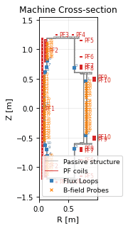
machine_geometry_poloidal · shot 39915 Stale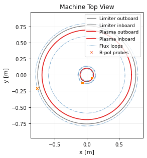
machine_geometry_topview · shot 39915 Stale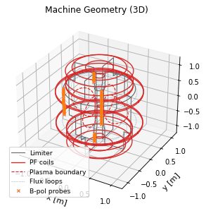
machine_geometry3d · shot 39915 Stalemachine_geometry_poloidal
geometry
source
machine / geometry / poloidal · domain machine · view model GeometryLayers
Composed poloidal machine view: wall, coils, passive structure and diagnostic positions and sight lines in one axes.
Interpretation
The machine’s poloidal cross-section in one axes: first wall and limiters, poloidal-field coils, passive conducting structure, and the positions and sight lines of the diagnostics. It is the map for locating a sensor relative to the plasma and coils, for reading other poloidal-plane figures, and for planning where a measurement looks.
Limitations
It is an axisymmetric projection: toroidally localized parts such as non-axisymmetric coils, ports and launchers appear at their poloidal position with their toroidal location lost. The geometry is drawn as the input’s machine description gives it, including any simplification in that description.
See Also
See Also
machine_geometry_topview : the same machine seen from above.
Thumbnail drawn from sample shot 39915, stale: renderer or style changed.
vaft.omas.plot_machine_geometry_poloidal(ods)         # from data
vaft.plot.machine_geometry_poloidal(model)   # from a GeometryLayers
Show source vaft/plot/renderers/geometry.py, lines 410–452
@_geometry_renderer(
    domain="machine", quantity="poloidal",
    subject="machine",
    description="Composed poloidal machine view: wall, coils, passive structure "
                "and diagnostic positions and sight lines in one axes.",
    ids=("wall", "pf_active", "pf_passive", "magnetics", "thomson_scattering",
         "charge_exchange", "soft_x_rays", "interferometer", "langmuir_probes"),
    required_paths=(),
    optional_paths=("wall.description_2d.{i}.limiter.unit.{j}.outline.r",
                    "pf_active.coil.{i}.element.{j}.geometry.geometry_type",
                    "pf_passive.loop.{i}.element.{j}.geometry.geometry_type"),
)
def machine_geometry_poloidal(
    model: GeometryLayers, *, ax: Axes | None = None, show: bool = False, **style: Any
) -> tuple[Figure, Axes]:
    """Composed poloidal machine view.

    Interpretation
    --------------
    The machine's poloidal cross-section in one axes: first wall and limiters,
    poloidal-field coils, passive conducting structure, and the positions and
    sight lines of the diagnostics.  It is the map for locating a sensor
    relative to the plasma and coils, for reading other poloidal-plane figures,
    and for planning where a measurement looks.

    Options
    -------
    ``overlay=`` selects which machine parts are drawn; with none named,
    everything the input describes is drawn.

    Limitations
    -----------
    It is an axisymmetric projection: toroidally localized parts such as
    non-axisymmetric coils, ports and launchers appear at their poloidal
    position with their toroidal location lost.  The geometry is drawn as the
    input's machine description gives it, including any simplification in that
    description.

    See Also
    --------
    machine_geometry_topview : the same machine seen from above.
    """
return render_geometry_layers(model, ax=ax, show=show, **style)| IDS | wall, pf_active, pf_passive, magnetics, thomson_scattering, charge_exchange, soft_x_rays, interferometer, langmuir_probes |
|---|---|
| Required paths | — |
| Optional paths | wall.description_2d.{i}.limiter.unit.{j}.outline.rpf_active.coil.{i}.element.{j}.geometry.geometry_typepf_passive.loop.{i}.element.{j}.geometry.geometry_type |
| Backends | matplotlib |
| Renderer | vaft.plot.renderers.geometry.machine_geometry_poloidal |
machine_geometry_topview
geometry
source
machine / geometry / topview · domain machine · view model GeometryLayers
Composed machine top view: machine-boundary and plasma extent, launcher, antenna and pellet-injector geometry, and the toroidal position of every diagnostic channel that stores one.
Thumbnail drawn from sample shot 39915, stale: renderer or style changed.
vaft.omas.plot_machine_geometry_topview(ods)         # from data
vaft.plot.machine_geometry_topview(model)   # from a GeometryLayers
Show source vaft/plot/renderers/geometry.py, lines 469–494
@_geometry_renderer(
    domain="machine", quantity="topview",
    subject="machine",
    description="Composed machine top view: machine-boundary and plasma extent, "
                "launcher, antenna and pellet-injector geometry, and the toroidal "
                "position of every diagnostic channel that stores one.",
    ids=("wall", "equilibrium", "lh_antennas", "ec_launchers", "pellets",
         "magnetics", "thomson_scattering", "charge_exchange", "langmuir_probes",
         "barometry", "interferometer", "soft_x_rays", "bolometer", "spectrometer_uv"),
    required_paths=(),
    optional_paths=("wall.description_2d.{i}.limiter.unit.{j}.outline.r",
                    "equilibrium.time_slice.{i}.boundary.outline.r",
                    "lh_antennas.antenna.{i}.position.r",
                    "ec_launchers.beam.{i}.launching_position.r",
                    "pellets.time_slice.{i}.pellet.{j}.path_geometry.first_point.r",
                    "magnetics.b_field_pol_probe.{i}.position.phi",
                    "magnetics.b_field_tor_probe.{i}.position.phi",
                    "magnetics.flux_loop.{i}.position.{j}.phi",
                    "thomson_scattering.channel.{i}.position.phi",
                    "soft_x_rays.channel.{i}.line_of_sight.first_point.phi"),
)
def machine_geometry_topview(
    model: GeometryLayers, *, ax: Axes | None = None, show: bool = False, **style: Any
) -> tuple[Figure, Axes]:
    """Composed machine top view."""
return render_geometry_layers(model, ax=ax, show=show, **style)| IDS | wall, equilibrium, lh_antennas, ec_launchers, pellets, magnetics, thomson_scattering, charge_exchange, langmuir_probes, barometry, interferometer, soft_x_rays, bolometer, spectrometer_uv |
|---|---|
| Required paths | — |
| Optional paths | wall.description_2d.{i}.limiter.unit.{j}.outline.requilibrium.time_slice.{i}.boundary.outline.rlh_antennas.antenna.{i}.position.rec_launchers.beam.{i}.launching_position.rpellets.time_slice.{i}.pellet.{j}.path_geometry.first_point.rmagnetics.b_field_pol_probe.{i}.position.phimagnetics.b_field_tor_probe.{i}.position.phimagnetics.flux_loop.{i}.position.{j}.phithomson_scattering.channel.{i}.position.phisoft_x_rays.channel.{i}.line_of_sight.first_point.phi |
| Backends | matplotlib |
| Renderer | vaft.plot.renderers.geometry.machine_geometry_topview |
machine_geometry3d
geometry3d
source
machine / geometry3d · domain machine · view model Geometry3DLayers
Composed 3D machine scene: wall and plasma-boundary cuts at four toroidal angles, PF coil rings, non-axisymmetric coils, and every diagnostic channel that stores r, phi and z.
Thumbnail drawn from sample shot 39915, stale: renderer or style changed.
vaft.omas.plot_machine_geometry3d(ods)         # from data
vaft.plot.machine_geometry3d(model)   # from a Geometry3DLayers
Show source vaft/plot/renderers/geometry.py, lines 590–611
@renderer(
    domain="machine", view="geometry3d", model=Geometry3DLayers,
    subject="machine",
    description="Composed 3D machine scene: wall and plasma-boundary cuts at four "
                "toroidal angles, PF coil rings, non-axisymmetric coils, and every "
                "diagnostic channel that stores r, phi and z.",
    ids=("wall", "pf_active", "coils_non_axisymmetric", "equilibrium", "magnetics",
         "thomson_scattering", "charge_exchange", "langmuir_probes", "barometry",
         "interferometer", "soft_x_rays", "bolometer", "spectrometer_uv"),
    required_paths=(),
    optional_paths=("wall.description_2d.{i}.limiter.unit.{j}.outline.r",
                    "pf_active.coil.{i}.element.{j}.geometry.geometry_type",
                    "coils_non_axisymmetric.coil.{i}.conductor.{j}.elements.start_points.r",
                    "equilibrium.time_slice.{i}.boundary.outline.r",
                    "magnetics.b_field_pol_probe.{i}.position.phi",
                    "soft_x_rays.channel.{i}.line_of_sight.first_point.phi"),
)
def machine_geometry3d(
    model: Geometry3DLayers, *, ax: Axes | None = None, show: bool = False, **style: Any
) -> tuple[Figure, Axes]:
    """Composed 3D machine scene."""
return render_geometry_3d_layers(model, ax=ax, show=show, **style)| IDS | wall, pf_active, coils_non_axisymmetric, equilibrium, magnetics, thomson_scattering, charge_exchange, langmuir_probes, barometry, interferometer, soft_x_rays, bolometer, spectrometer_uv |
|---|---|
| Required paths | — |
| Optional paths | wall.description_2d.{i}.limiter.unit.{j}.outline.rpf_active.coil.{i}.element.{j}.geometry.geometry_typecoils_non_axisymmetric.coil.{i}.conductor.{j}.elements.start_points.requilibrium.time_slice.{i}.boundary.outline.rmagnetics.b_field_pol_probe.{i}.position.phisoft_x_rays.channel.{i}.line_of_sight.first_point.phi |
| Backends | matplotlib, plotly |
| Renderer | vaft.plot.renderers.geometry.machine_geometry3d |
nbi [neutral_beam, nubeam]
nbi_profile_current_drivenbi_profile_electron_heatingnbi_profile_ion_heatingnbi_profile_current_drive
profile
source
nbi / profile / current_drive · domain core_sources · view model Profile1D
Beam-driven parallel current density against normalized toroidal flux, <J.B>/B0. Derived from the solver's toroidal driven current and the equilibrium geometry, assuming the driven current is field-aligned on each flux surface; it is not a direct solver output.
No thumbnail: no packaged sample carries the data this plot needs.
vaft.omas.plot_nbi_profile_current_drive(ods)         # from data
vaft.plot.nbi_profile_current_drive(model)   # from a Profile1D
Show source vaft/plot/renderers/profiles.py, lines 985–1003
@_profile_renderer(
    domain="core_sources", quantity="current_drive",
    subject="nbi",
    description="Beam-driven parallel current density against normalized toroidal "
                "flux, <J.B>/B0. Derived from the solver's toroidal driven current "
                "and the equilibrium geometry, assuming the driven current is "
                "field-aligned on each flux surface; it is not a direct solver "
                "output.",
    ids=("core_sources",),
    required_paths=_NBI_PROFILE_PATHS + (
        "core_sources.source.{i}.profiles_1d.{j}.j_parallel",
    ),
    optional_paths=("core_sources.source.{i}.profiles_1d.{j}.current_parallel_inside",),
)
def nbi_profile_current_drive(
    model: Profile1D, *, ax: Axes | None = None, show: bool = False, **style: Any
) -> tuple[Figure, Axes]:
    """Beam-driven parallel current density."""
return render_profile_1d(model, ax=ax, show=show, **style)| IDS | core_sources |
|---|---|
| Required paths | core_sources.source.{i}.identifier.indexcore_sources.source.{i}.profiles_1d.{j}.grid.rho_tor_normcore_sources.source.{i}.profiles_1d.{j}.j_parallel |
| Optional paths | core_sources.source.{i}.profiles_1d.{j}.current_parallel_inside |
| Backends | matplotlib, plotly |
| Renderer | vaft.plot.renderers.profiles.nbi_profile_current_drive |
nbi_profile_electron_heating
profile
source
nbi / profile / electron_heating · domain core_sources · view model Profile1D
Beam power density to electrons against normalized toroidal flux, from a NUBEAM result mapped into core_sources.
No thumbnail: no packaged sample carries the data this plot needs.
vaft.omas.plot_nbi_profile_electron_heating(ods)         # from data
vaft.plot.nbi_profile_electron_heating(model)   # from a Profile1D
Show source vaft/plot/renderers/profiles.py, lines 949–964
@_profile_renderer(
    domain="core_sources", quantity="electron_heating",
    subject="nbi",
    description="Beam power density to electrons against normalized toroidal flux, "
                "from a NUBEAM result mapped into core_sources.",
    ids=("core_sources",),
    required_paths=_NBI_PROFILE_PATHS + (
        "core_sources.source.{i}.profiles_1d.{j}.electrons.energy",
    ),
    optional_paths=("core_sources.source.{i}.profiles_1d.{j}.electrons.power_inside",),
)
def nbi_profile_electron_heating(
    model: Profile1D, *, ax: Axes | None = None, show: bool = False, **style: Any
) -> tuple[Figure, Axes]:
    """Beam power density to electrons."""
return render_profile_1d(model, ax=ax, show=show, **style)| IDS | core_sources |
|---|---|
| Required paths | core_sources.source.{i}.identifier.indexcore_sources.source.{i}.profiles_1d.{j}.grid.rho_tor_normcore_sources.source.{i}.profiles_1d.{j}.electrons.energy |
| Optional paths | core_sources.source.{i}.profiles_1d.{j}.electrons.power_inside |
| Backends | matplotlib, plotly |
| Renderer | vaft.plot.renderers.profiles.nbi_profile_electron_heating |
nbi_profile_ion_heating
profile
source
nbi / profile / ion_heating · domain core_sources · view model Profile1D
Beam power density to ions against normalized toroidal flux, from a NUBEAM result mapped into core_sources.
No thumbnail: no packaged sample carries the data this plot needs.
vaft.omas.plot_nbi_profile_ion_heating(ods)         # from data
vaft.plot.nbi_profile_ion_heating(model)   # from a Profile1D
Show source vaft/plot/renderers/profiles.py, lines 967–982
@_profile_renderer(
    domain="core_sources", quantity="ion_heating",
    subject="nbi",
    description="Beam power density to ions against normalized toroidal flux, from "
                "a NUBEAM result mapped into core_sources.",
    ids=("core_sources",),
    required_paths=_NBI_PROFILE_PATHS + (
        "core_sources.source.{i}.profiles_1d.{j}.total_ion_energy",
    ),
    optional_paths=("core_sources.source.{i}.profiles_1d.{j}.total_ion_power_inside",),
)
def nbi_profile_ion_heating(
    model: Profile1D, *, ax: Axes | None = None, show: bool = False, **style: Any
) -> tuple[Figure, Axes]:
    """Beam power density to ions."""
return render_profile_1d(model, ax=ax, show=show, **style)| IDS | core_sources |
|---|---|
| Required paths | core_sources.source.{i}.identifier.indexcore_sources.source.{i}.profiles_1d.{j}.grid.rho_tor_normcore_sources.source.{i}.profiles_1d.{j}.total_ion_energy |
| Optional paths | core_sources.source.{i}.profiles_1d.{j}.total_ion_power_inside |
| Backends | matplotlib, plotly |
| Renderer | vaft.plot.renderers.profiles.nbi_profile_ion_heating |
ec_launchers [ech, ecrh, electron_cyclotron]
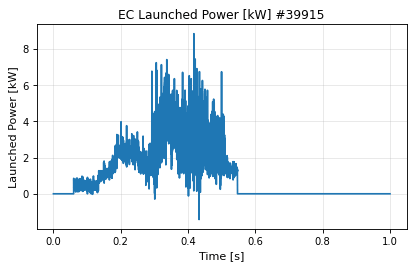
ec_launchers_time_power · shot 39915 Staleec_launchers_time_power
time
source
ec_launchers / time / power · domain ec_launchers · view model LineSeries
Net launched electron-cyclotron power (forward minus reflected) per beam; noisy, so smooth= is a rolling median in seconds.
Thumbnail drawn from sample shot 39915, stale: renderer or style changed.
vaft.omas.plot_ec_launchers_time_power(ods)         # from data
vaft.plot.ec_launchers_time_power(model)   # from a LineSeries
Show source vaft/plot/renderers/lines.py, lines 1249–1272
@renderer(
    domain="ec_launchers",
    subject="ec_launchers",
    view="time",
    quantity="power",
    model=LineSeries,
    description="Net launched electron-cyclotron power (forward minus reflected) per beam; "
                "noisy, so smooth= is a rolling median in seconds.",
    ids=("ec_launchers",),
    required_paths=("ec_launchers.beam.{i}.power_launched.data",),
    optional_paths=(
        "ec_launchers.beam.{i}.power_launched.time",
        "ec_launchers.beam.{i}.name",
    ),
)
def ec_launchers_time_power(
    model: LineSeries,
    *,
    ax: Axes | None = None,
    show: bool = False,
    **style: Any,
) -> tuple[Figure, Axes]:
    """Net launched electron-cyclotron power per beam."""
return render_line_series(model, ax=ax, show=show, **style)| IDS | ec_launchers |
|---|---|
| Required paths | ec_launchers.beam.{i}.power_launched.data |
| Optional paths | ec_launchers.beam.{i}.power_launched.timeec_launchers.beam.{i}.name |
| Backends | matplotlib, plotly |
| Renderer | vaft.plot.renderers.lines.ec_launchers_time_power |
Reconstruction subjects
equilibrium
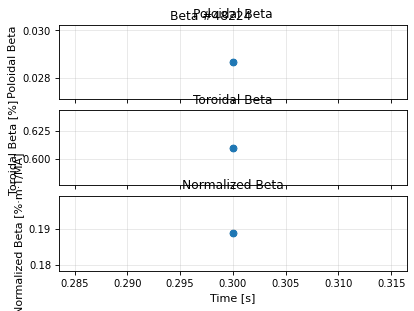
equilibrium_time_beta · shot 48224 Stale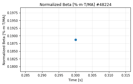
equilibrium_time_beta_n · shot 48224 Stale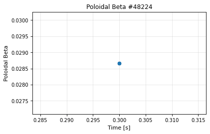
equilibrium_time_beta_p · shot 48224 Stale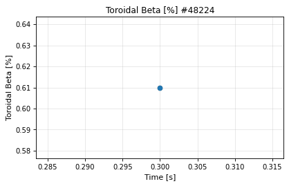
equilibrium_time_beta_t · shot 48224 Stale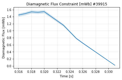
equilibrium_time_diamagnetic_flux · shot 39915 Staleequilibrium_time_elongation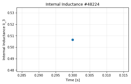
equilibrium_time_li · shot 48224 Staleequilibrium_time_major_radiusequilibrium_time_minor_radius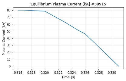
equilibrium_time_plasma_current · shot 39915 Stale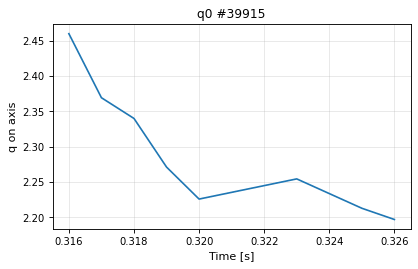
equilibrium_time_q0 · shot 39915 Stale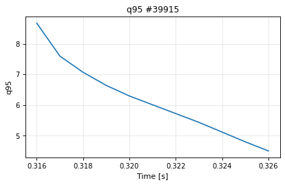
equilibrium_time_q95 · shot 39915 Staleequilibrium_time_qaequilibrium_time_shapeequilibrium_time_triangularityequilibrium_time_triangularity_lowerequilibrium_time_triangularity_upper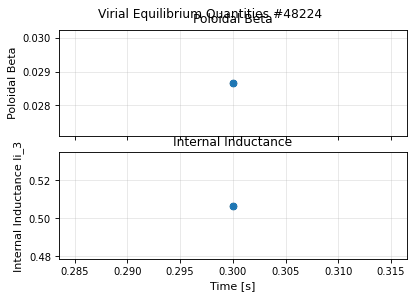
equilibrium_time_virial · shot 48224 Staleequilibrium_time_w_magequilibrium_time_w_mhdequilibrium_time_w_tot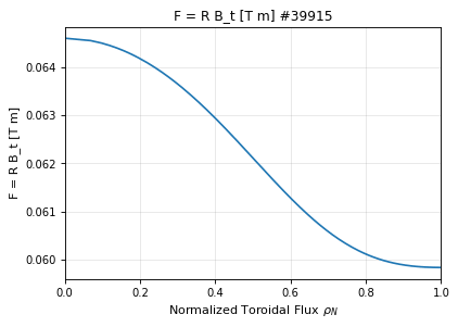
equilibrium_profile_f · shot 39915 Stale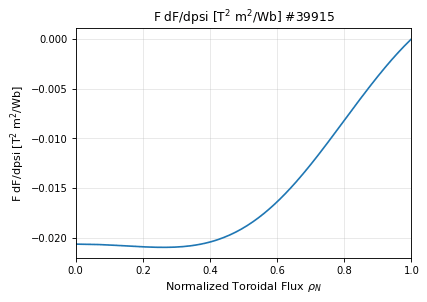
equilibrium_profile_ffprime · shot 39915 Stale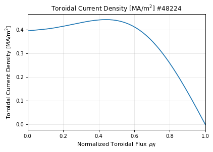
equilibrium_profile_j_tor · shot 48224 Stale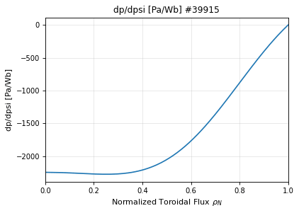
equilibrium_profile_pprime · shot 39915 Stale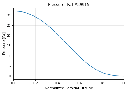
equilibrium_profile_pressure · shot 39915 Stale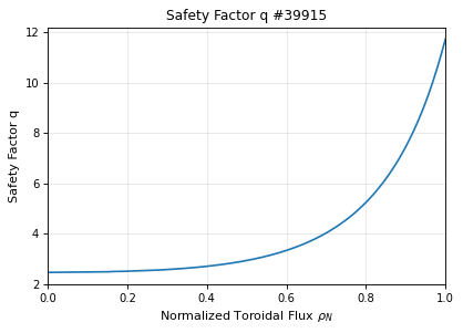
equilibrium_profile_q · shot 39915 Stale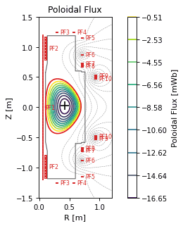
equilibrium_field_2d · shot 39915 Stale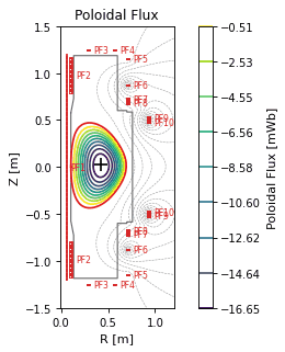
equilibrium_field_psi · shot 39915 Stale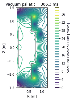
equilibrium_field_psi_vacuum · shot 39915 Stale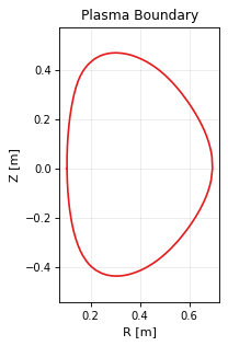
equilibrium_geometry_boundary · shot 39915 Stale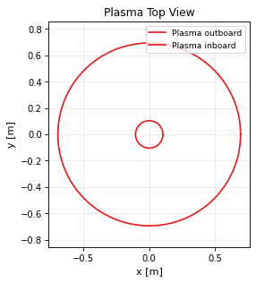
equilibrium_geometry_topview · shot 39915 Stale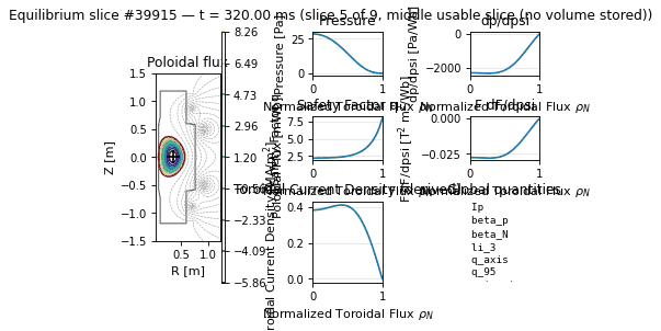
equilibrium_overview · shot 39915 Stale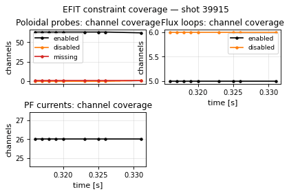
equilibrium_overview_constraint_coverage · shot 39915 Stale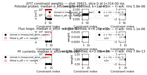
equilibrium_overview_constraint_weights · shot 39915 Stale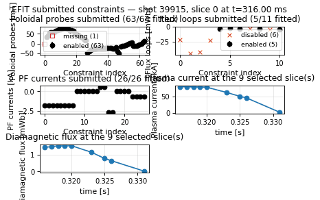
equilibrium_overview_constraints · shot 39915 Stale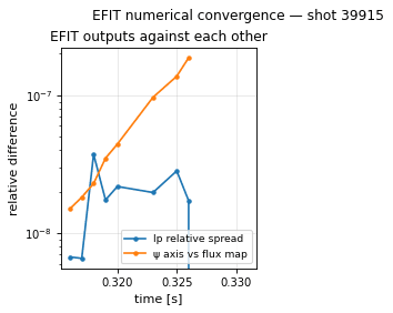
equilibrium_overview_convergence · shot 39915 Stale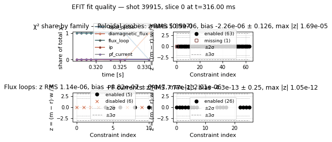
equilibrium_overview_fit_quality · shot 39915 Stale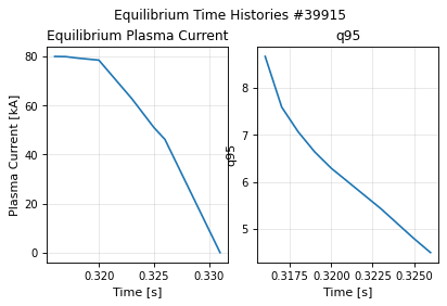
equilibrium_overview_histories · shot 39915 Stale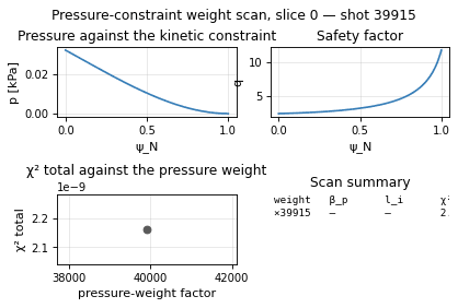
equilibrium_overview_pressure_weight_scan · shot 39915 Stale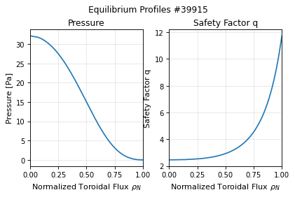
equilibrium_overview_profiles · shot 39915 Stale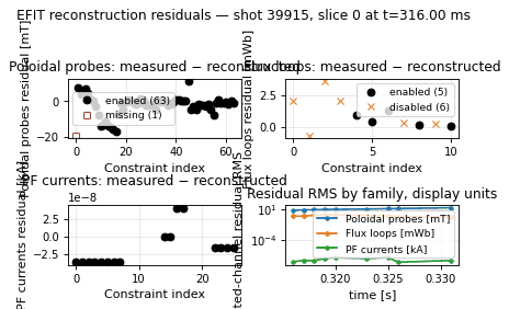
equilibrium_overview_residuals · shot 39915 Stale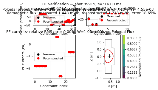
equilibrium_overview_verification · shot 39915 Staleequilibrium_table_fit_qualityequilibrium_table_summaryequilibrium_table_validationequilibrium_text_summaryequilibrium_time_beta
time
source
equilibrium / time / beta · domain equilibrium · view model Panels
Poloidal, toroidal and normalized beta panels.
Interpretation
The three common measures of plasma pressure relative to magnetic pressure against time, one panel each, from the reconstruction’s slices: poloidal beta (against the poloidal field of the plasma current), toroidal beta (against the vacuum toroidal field at the reference radius) and normalized beta (the toroidal beta in percent scaled by a B0 / I_p, the Troyon normalization). Read together they follow how heating and confinement raise the pressure and how close the discharge comes to the pressure the field can confine.
Limitations
Beta is a reconstruction output. With magnetic constraints alone, poloidal beta and the internal inductance are not separately well determined – mainly their sum beta_p + l_i / 2 is – particularly for nearly circular plasmas; a diamagnetic or kinetic pressure constraint improves it. Proximity to an empirical beta limit is context, not a stability verdict: the actual limit depends on the profiles, the shape and the wall.
See Also
See Also
equilibrium_time_beta_p : poloidal beta alone. equilibrium_time_beta_n : normalized beta alone.
Thumbnail drawn from sample shot 48224, stale: renderer or style changed.
vaft.omas.plot_equilibrium_time_beta(ods)         # from data
vaft.plot.equilibrium_time_beta(model)   # from a Panels
Show source vaft/plot/renderers/panels.py, lines 600–639
@_panel_renderer(
    domain="equilibrium",
    subject="equilibrium",
    view="time",
    quantity="beta",
    description="Poloidal, toroidal and normalized beta panels.",
    ids=("equilibrium",),
    required_paths=("equilibrium.time_slice.{i}.global_quantities.beta_pol",),
)
def equilibrium_time_beta(
    model: Panels, *, ax: Any = None, show: bool = False, **style: Any
) -> tuple[Figure, np.ndarray]:
    """Poloidal, toroidal and normalized beta panels.

    Interpretation
    --------------
    The three common measures of plasma pressure relative to magnetic pressure
    against time, one panel each, from the reconstruction's slices: poloidal
    beta (against the poloidal field of the plasma current), toroidal beta
    (against the vacuum toroidal field at the reference radius) and normalized
    beta (the toroidal beta in percent scaled by a B0 / I_p, the Troyon
    normalization). Read together they follow how heating and confinement raise
    the pressure and how close the discharge comes to the pressure the field
    can confine.

    Limitations
    -----------
    Beta is a reconstruction output.  With magnetic constraints alone, poloidal
    beta and the internal inductance are not separately well determined --
    mainly their sum beta_p + l_i / 2 is -- particularly for nearly circular
    plasmas; a diamagnetic or kinetic pressure constraint improves it.
    Proximity to an empirical beta limit is context, not a stability verdict:
    the actual limit depends on the profiles, the shape and the wall.

    See Also
    --------
    equilibrium_time_beta_p : poloidal beta alone.
    equilibrium_time_beta_n : normalized beta alone.
    """
return render_panels(model, ax=ax, show=show, **style)| IDS | equilibrium |
|---|---|
| Required paths | equilibrium.time_slice.{i}.global_quantities.beta_pol |
| Backends | matplotlib, plotly |
| Renderer | vaft.plot.renderers.panels.equilibrium_time_beta |
equilibrium_time_beta_n
time
source
equilibrium / time / beta_n · domain equilibrium · view model LineSeries
Normalized beta history.
Interpretation
Normalized beta beta_N = beta_t[%] a B0 / I_p[MA] at each reconstructed slice: the toroidal beta scaled by the Troyon normalization, which removes most of the dependence on current and field and so compares discharges of different current and field on one scale. It is the usual ordinate for judging how close a plasma comes to ideal pressure-driven limits.
Limitations
Beta is a reconstruction output. With magnetic constraints alone, poloidal beta and the internal inductance are not separately well determined – mainly their sum beta_p + l_i / 2 is – particularly for nearly circular plasmas; a diamagnetic or kinetic pressure constraint improves it. Proximity to an empirical beta limit is context, not a stability verdict: the actual limit depends on the profiles, the shape and the wall.
See Also
See Also
equilibrium_time_beta : beta_p, beta_t and beta_N together.
Thumbnail drawn from sample shot 48224, stale: renderer or style changed.
vaft.omas.plot_equilibrium_time_beta_n(ods)         # from data
vaft.plot.equilibrium_time_beta_n(model)   # from a LineSeries
Show source vaft/plot/renderers/lines.py, lines 755–799
@renderer(
    domain="equilibrium",
    subject="equilibrium",
    view="time",
    quantity="beta_n",
    model=LineSeries,
    description="Normalized beta history.",
    ids=("equilibrium",),
    required_paths=(
        "equilibrium.time",
        "equilibrium.time_slice.{i}.global_quantities.beta_normal",
    ),
    optional_paths=(),
)
def equilibrium_time_beta_n(
    model: LineSeries,
    *,
    ax: Axes | None = None,
    show: bool = False,
    **style: Any,
) -> tuple[Figure, Axes]:
    """Normalized beta history.

    Interpretation
    --------------
    Normalized beta beta_N = beta_t[%] a B0 / I_p[MA] at each reconstructed
    slice: the toroidal beta scaled by the Troyon normalization, which removes
    most of the dependence on current and field and so compares discharges of
    different current and field on one scale.  It is the usual ordinate for
    judging how close a plasma comes to ideal pressure-driven limits.

    Limitations
    -----------
    Beta is a reconstruction output.  With magnetic constraints alone, poloidal
    beta and the internal inductance are not separately well determined --
    mainly their sum beta_p + l_i / 2 is -- particularly for nearly circular
    plasmas; a diamagnetic or kinetic pressure constraint improves it.
    Proximity to an empirical beta limit is context, not a stability verdict:
    the actual limit depends on the profiles, the shape and the wall.

    See Also
    --------
    equilibrium_time_beta : beta_p, beta_t and beta_N together.
    """
return render_line_series(model, ax=ax, show=show, **style)| IDS | equilibrium |
|---|---|
| Required paths | equilibrium.timeequilibrium.time_slice.{i}.global_quantities.beta_normal |
| Backends | matplotlib, plotly |
| Renderer | vaft.plot.renderers.lines.equilibrium_time_beta_n |
equilibrium_time_beta_p
time
source
equilibrium / time / beta_p · domain equilibrium · view model LineSeries
Poloidal beta history.
Interpretation
Poloidal beta at each reconstructed slice: the volume-averaged plasma pressure relative to the magnetic pressure of the poloidal field produced by the plasma current. It measures how much pressure the plasma current confines, and enters the Shafranov shift and the vertical field needed for radial equilibrium. beta_p near 1 separates a diamagnetic from a paramagnetic plasma.
Limitations
Beta is a reconstruction output. With magnetic constraints alone, poloidal beta and the internal inductance are not separately well determined – mainly their sum beta_p + l_i / 2 is – particularly for nearly circular plasmas; a diamagnetic or kinetic pressure constraint improves it. Proximity to an empirical beta limit is context, not a stability verdict: the actual limit depends on the profiles, the shape and the wall.
See Also
See Also
diamagnetic_flux_time : the measurement most directly related to beta_p. equilibrium_time_li : the internal inductance it is entangled with.
Thumbnail drawn from sample shot 48224, stale: renderer or style changed.
vaft.omas.plot_equilibrium_time_beta_p(ods)         # from data
vaft.plot.equilibrium_time_beta_p(model)   # from a LineSeries
Show source vaft/plot/renderers/lines.py, lines 659–705
@renderer(
    domain="equilibrium",
    subject="equilibrium",
    view="time",
    quantity="beta_p",
    model=LineSeries,
    description="Poloidal beta history.",
    ids=("equilibrium",),
    required_paths=(
        "equilibrium.time",
        "equilibrium.time_slice.{i}.global_quantities.beta_pol",
    ),
    optional_paths=(),
)
def equilibrium_time_beta_p(
    model: LineSeries,
    *,
    ax: Axes | None = None,
    show: bool = False,
    **style: Any,
) -> tuple[Figure, Axes]:
    """Poloidal beta history.

    Interpretation
    --------------
    Poloidal beta at each reconstructed slice: the volume-averaged plasma
    pressure relative to the magnetic pressure of the poloidal field produced
    by the plasma current.  It measures how much pressure the plasma current
    confines, and enters the Shafranov shift and the vertical field needed for
    radial equilibrium.  beta_p near 1 separates a diamagnetic from a
    paramagnetic plasma.

    Limitations
    -----------
    Beta is a reconstruction output.  With magnetic constraints alone, poloidal
    beta and the internal inductance are not separately well determined --
    mainly their sum beta_p + l_i / 2 is -- particularly for nearly circular
    plasmas; a diamagnetic or kinetic pressure constraint improves it.
    Proximity to an empirical beta limit is context, not a stability verdict:
    the actual limit depends on the profiles, the shape and the wall.

    See Also
    --------
    diamagnetic_flux_time : the measurement most directly related to beta_p.
    equilibrium_time_li : the internal inductance it is entangled with.
    """
return render_line_series(model, ax=ax, show=show, **style)| IDS | equilibrium |
|---|---|
| Required paths | equilibrium.timeequilibrium.time_slice.{i}.global_quantities.beta_pol |
| Backends | matplotlib, plotly |
| Renderer | vaft.plot.renderers.lines.equilibrium_time_beta_p |
equilibrium_time_beta_t
time
source
equilibrium / time / beta_t · domain equilibrium · view model LineSeries
Toroidal beta history.
Interpretation
Toroidal beta at each reconstructed slice: the volume-averaged plasma pressure relative to the magnetic pressure of the vacuum toroidal field at the reference radius. It measures how efficiently the toroidal field confines pressure; a reactor’s fusion power density scales as beta_t^2 B^4 at fixed temperature.
Limitations
Beta is a reconstruction output. With magnetic constraints alone, poloidal beta and the internal inductance are not separately well determined – mainly their sum beta_p + l_i / 2 is – particularly for nearly circular plasmas; a diamagnetic or kinetic pressure constraint improves it. Proximity to an empirical beta limit is context, not a stability verdict: the actual limit depends on the profiles, the shape and the wall.
See Also
See Also
equilibrium_time_beta_n : toroidal beta on the Troyon scale.
Thumbnail drawn from sample shot 48224, stale: renderer or style changed.
vaft.omas.plot_equilibrium_time_beta_t(ods)         # from data
vaft.plot.equilibrium_time_beta_t(model)   # from a LineSeries
Show source vaft/plot/renderers/lines.py, lines 708–752
@renderer(
    domain="equilibrium",
    subject="equilibrium",
    view="time",
    quantity="beta_t",
    model=LineSeries,
    description="Toroidal beta history.",
    ids=("equilibrium",),
    required_paths=(
        "equilibrium.time",
        "equilibrium.time_slice.{i}.global_quantities.beta_tor",
    ),
    optional_paths=(),
)
def equilibrium_time_beta_t(
    model: LineSeries,
    *,
    ax: Axes | None = None,
    show: bool = False,
    **style: Any,
) -> tuple[Figure, Axes]:
    """Toroidal beta history.

    Interpretation
    --------------
    Toroidal beta at each reconstructed slice: the volume-averaged plasma
    pressure relative to the magnetic pressure of the vacuum toroidal field at
    the reference radius.  It measures how efficiently the toroidal field
    confines pressure; a reactor's fusion power density scales as beta_t^2 B^4
    at fixed temperature.

    Limitations
    -----------
    Beta is a reconstruction output.  With magnetic constraints alone, poloidal
    beta and the internal inductance are not separately well determined --
    mainly their sum beta_p + l_i / 2 is -- particularly for nearly circular
    plasmas; a diamagnetic or kinetic pressure constraint improves it.
    Proximity to an empirical beta limit is context, not a stability verdict:
    the actual limit depends on the profiles, the shape and the wall.

    See Also
    --------
    equilibrium_time_beta_n : toroidal beta on the Troyon scale.
    """
return render_line_series(model, ax=ax, show=show, **style)| IDS | equilibrium |
|---|---|
| Required paths | equilibrium.timeequilibrium.time_slice.{i}.global_quantities.beta_tor |
| Backends | matplotlib, plotly |
| Renderer | vaft.plot.renderers.lines.equilibrium_time_beta_t |
equilibrium_time_diamagnetic_flux
time
source
equilibrium / time / diamagnetic_flux · domain equilibrium · view model LineSeries
Measured versus reconstructed diamagnetic-flux constraint.
Thumbnail drawn from sample shot 39915, stale: renderer or style changed.
vaft.omas.plot_equilibrium_time_diamagnetic_flux(ods)         # from data
vaft.plot.equilibrium_time_diamagnetic_flux(model)   # from a LineSeries
Show source vaft/plot/renderers/lines.py, lines 1124–1146
@renderer(
    domain="equilibrium",
    subject="equilibrium",
    view="time",
    quantity="diamagnetic_flux",
    model=LineSeries,
    description="Measured versus reconstructed diamagnetic-flux constraint.",
    ids=("equilibrium",),
    required_paths=("equilibrium.time",),
    optional_paths=(
        "equilibrium.time_slice.{i}.constraints.diamagnetic_flux.measured",
        "equilibrium.time_slice.{i}.constraints.diamagnetic_flux.reconstructed",
    ),
)
def equilibrium_time_diamagnetic_flux(
    model: LineSeries,
    *,
    ax: Axes | None = None,
    show: bool = False,
    **style: Any,
) -> tuple[Figure, Axes]:
    """Measured versus reconstructed diamagnetic-flux constraint."""
return render_line_series(model, ax=ax, show=show, **style)| IDS | equilibrium |
|---|---|
| Required paths | equilibrium.time |
| Optional paths | equilibrium.time_slice.{i}.constraints.diamagnetic_flux.measuredequilibrium.time_slice.{i}.constraints.diamagnetic_flux.reconstructed |
| Backends | matplotlib, plotly |
| Renderer | vaft.plot.renderers.lines.equilibrium_time_diamagnetic_flux |
equilibrium_time_elongation
time
source
equilibrium / time / elongation · domain equilibrium · view model LineSeries
Boundary elongation history.
No thumbnail: no packaged sample carries the data this plot needs.
vaft.omas.plot_equilibrium_time_elongation(ods)         # from data
vaft.plot.equilibrium_time_elongation(model)   # from a LineSeries
Show source vaft/plot/renderers/lines.py, lines 999–1021
@renderer(
domain="equilibrium",
subject="equilibrium",
view="time",
quantity="elongation",
model=LineSeries,
description="Boundary elongation history.",
ids=("equilibrium",),
required_paths=(
"equilibrium.time",
"equilibrium.time_slice.{i}.boundary.elongation",
),
optional_paths=(),
)
def equilibrium_time_elongation(
model: LineSeries,
*,
ax: Axes | None = None,
show: bool = False,
**style: Any,
) -> tuple[Figure, Axes]:
"""Boundary elongation history."""
return render_line_series(model, ax=ax, show=show, **style)| IDS | equilibrium |
|---|---|
| Required paths | equilibrium.timeequilibrium.time_slice.{i}.boundary.elongation |
| Backends | matplotlib, plotly |
| Renderer | vaft.plot.renderers.lines.equilibrium_time_elongation |
equilibrium_time_li
time
source
equilibrium / time / li · domain equilibrium · view model LineSeries
Internal inductance li_3 history.
Thumbnail drawn from sample shot 48224, stale: renderer or style changed.
vaft.omas.plot_equilibrium_time_li(ods) # from data
vaft.plot.equilibrium_time_li(model) # from a LineSeriesShow source vaft/plot/renderers/lines.py, lines 634–656
@renderer(
domain="equilibrium",
subject="equilibrium",
view="time",
quantity="li",
model=LineSeries,
description="Internal inductance li_3 history.",
ids=("equilibrium",),
required_paths=(
"equilibrium.time",
"equilibrium.time_slice.{i}.global_quantities.li_3",
),
optional_paths=(),
)
def equilibrium_time_li(
model: LineSeries,
*,
ax: Axes | None = None,
show: bool = False,
**style: Any,
) -> tuple[Figure, Axes]:
"""Internal inductance li_3 history."""
return render_line_series(model, ax=ax, show=show, **style)| IDS | equilibrium |
|---|---|
| Required paths | equilibrium.timeequilibrium.time_slice.{i}.global_quantities.li_3 |
| Backends | matplotlib, plotly |
| Renderer | vaft.plot.renderers.lines.equilibrium_time_li |
equilibrium_time_major_radius
time
source
equilibrium / time / major_radius · domain equilibrium · view model LineSeries
Geometric-axis major radius history.
No thumbnail: no packaged sample carries the data this plot needs.
vaft.omas.plot_equilibrium_time_major_radius(ods) # from data
vaft.plot.equilibrium_time_major_radius(model) # from a LineSeriesShow source vaft/plot/renderers/lines.py, lines 1099–1121
@renderer(
domain="equilibrium",
subject="equilibrium",
view="time",
quantity="major_radius",
model=LineSeries,
description="Geometric-axis major radius history.",
ids=("equilibrium",),
required_paths=(
"equilibrium.time",
"equilibrium.time_slice.{i}.boundary.geometric_axis.r",
),
optional_paths=(),
)
def equilibrium_time_major_radius(
model: LineSeries,
*,
ax: Axes | None = None,
show: bool = False,
**style: Any,
) -> tuple[Figure, Axes]:
"""Geometric-axis major radius history."""
return render_line_series(model, ax=ax, show=show, **style)| IDS | equilibrium |
|---|---|
| Required paths | equilibrium.timeequilibrium.time_slice.{i}.boundary.geometric_axis.r |
| Backends | matplotlib, plotly |
| Renderer | vaft.plot.renderers.lines.equilibrium_time_major_radius |
equilibrium_time_minor_radius
time
source
equilibrium / time / minor_radius · domain equilibrium · view model LineSeries
Boundary minor radius history.
No thumbnail: no packaged sample carries the data this plot needs.
vaft.omas.plot_equilibrium_time_minor_radius(ods) # from data
vaft.plot.equilibrium_time_minor_radius(model) # from a LineSeriesShow source vaft/plot/renderers/lines.py, lines 974–996
@renderer(
domain="equilibrium",
subject="equilibrium",
view="time",
quantity="minor_radius",
model=LineSeries,
description="Boundary minor radius history.",
ids=("equilibrium",),
required_paths=(
"equilibrium.time",
"equilibrium.time_slice.{i}.boundary.minor_radius",
),
optional_paths=(),
)
def equilibrium_time_minor_radius(
model: LineSeries,
*,
ax: Axes | None = None,
show: bool = False,
**style: Any,
) -> tuple[Figure, Axes]:
"""Boundary minor radius history."""
return render_line_series(model, ax=ax, show=show, **style)| IDS | equilibrium |
|---|---|
| Required paths | equilibrium.timeequilibrium.time_slice.{i}.boundary.minor_radius |
| Backends | matplotlib, plotly |
| Renderer | vaft.plot.renderers.lines.equilibrium_time_minor_radius |
equilibrium_time_plasma_current
time
source
equilibrium / time / plasma_current · domain equilibrium · view model LineSeries
Reconstructed plasma current history.
Thumbnail drawn from sample shot 39915, stale: renderer or style changed.
vaft.omas.plot_equilibrium_time_plasma_current(ods) # from data
vaft.plot.equilibrium_time_plasma_current(model) # from a LineSeriesShow source vaft/plot/renderers/lines.py, lines 609–631
@renderer(
domain="equilibrium",
subject="equilibrium",
view="time",
quantity="plasma_current",
model=LineSeries,
description="Reconstructed plasma current history.",
ids=("equilibrium",),
required_paths=(
"equilibrium.time",
"equilibrium.time_slice.{i}.global_quantities.ip",
),
optional_paths=(),
)
def equilibrium_time_plasma_current(
model: LineSeries,
*,
ax: Axes | None = None,
show: bool = False,
**style: Any,
) -> tuple[Figure, Axes]:
"""Reconstructed plasma current history."""
return render_line_series(model, ax=ax, show=show, **style)| IDS | equilibrium |
|---|---|
| Required paths | equilibrium.timeequilibrium.time_slice.{i}.global_quantities.ip |
| Backends | matplotlib, plotly |
| Renderer | vaft.plot.renderers.lines.equilibrium_time_plasma_current |
equilibrium_time_q0
time
source
equilibrium / time / q0 · domain equilibrium · view model LineSeries
Safety factor on axis.
Thumbnail drawn from sample shot 39915, stale: renderer or style changed.
vaft.omas.plot_equilibrium_time_q0(ods) # from data
vaft.plot.equilibrium_time_q0(model) # from a LineSeriesShow source vaft/plot/renderers/lines.py, lines 877–899
@renderer(
domain="equilibrium",
subject="equilibrium",
view="time",
quantity="q0",
model=LineSeries,
description="Safety factor on axis.",
ids=("equilibrium",),
required_paths=(
"equilibrium.time",
"equilibrium.time_slice.{i}.global_quantities.q_axis",
),
optional_paths=(),
)
def equilibrium_time_q0(
model: LineSeries,
*,
ax: Axes | None = None,
show: bool = False,
**style: Any,
) -> tuple[Figure, Axes]:
"""Safety factor on axis."""
return render_line_series(model, ax=ax, show=show, **style)| IDS | equilibrium |
|---|---|
| Required paths | equilibrium.timeequilibrium.time_slice.{i}.global_quantities.q_axis |
| Backends | matplotlib, plotly |
| Renderer | vaft.plot.renderers.lines.equilibrium_time_q0 |
equilibrium_time_q95
time
source
equilibrium / time / q95 · domain equilibrium · view model LineSeries
Safety factor at the 95% flux surface.
Interpretation
q95, the safety factor on the flux surface enclosing 95 % of the poloidal flux, at each reconstructed slice. It summarizes the edge field-line pitch – the plasma current relative to the toroidal field and the shape – in one number that stays finite for a diverted plasma, and is the usual coordinate for the low-q operating boundary: discharges approaching q95 of about 2 meet the external-kink limit and disrupt more often.
Limitations
q95 exists only where a reconstruction exists; the line between slice markers joins them visually and is not a reconstruction. Its accuracy is the equilibrium’s: it depends on the boundary and the current-profile parametrisation.
See Also
See Also
summary_time_estimated_q95 : a q95 estimated from scalings without a reconstruction. equilibrium_profile_q : the whole q profile at one slice.
Thumbnail drawn from sample shot 39915, stale: renderer or style changed.
vaft.omas.plot_equilibrium_time_q95(ods) # from data
vaft.plot.equilibrium_time_q95(model) # from a LineSeriesShow source vaft/plot/renderers/lines.py, lines 902–946
@renderer(
domain="equilibrium",
subject="equilibrium",
view="time",
quantity="q95",
model=LineSeries,
description="Safety factor at the 95% flux surface.",
ids=("equilibrium",),
required_paths=(
"equilibrium.time",
"equilibrium.time_slice.{i}.global_quantities.q_95",
),
optional_paths=(),
)
def equilibrium_time_q95(
model: LineSeries,
*,
ax: Axes | None = None,
show: bool = False,
**style: Any,
) -> tuple[Figure, Axes]:
"""Safety factor at the 95% flux surface.
Interpretation
--------------
q95, the safety factor on the flux surface enclosing 95 % of the poloidal
flux, at each reconstructed slice. It summarizes the edge field-line pitch
-- the plasma current relative to the toroidal field and the shape -- in
one number that stays finite for a diverted plasma, and is the usual
coordinate for the low-q operating boundary: discharges approaching q95 of
about 2 meet the external-kink limit and disrupt more often.
Limitations
-----------
q95 exists only where a reconstruction exists; the line between slice
markers joins them visually and is not a reconstruction. Its accuracy is
the equilibrium's: it depends on the boundary and the current-profile
parametrisation.
See Also
--------
summary_time_estimated_q95 : a q95 estimated from scalings without a reconstruction.
equilibrium_profile_q : the whole q profile at one slice.
"""
return render_line_series(model, ax=ax, show=show, **style)| IDS | equilibrium |
|---|---|
| Required paths | equilibrium.timeequilibrium.time_slice.{i}.global_quantities.q_95 |
| Backends | matplotlib, plotly |
| Renderer | vaft.plot.renderers.lines.equilibrium_time_q95 |
equilibrium_time_qa
time
source
equilibrium / time / qa · domain equilibrium · view model LineSeries
Safety factor at the plasma edge.
No thumbnail: no packaged sample carries the data this plot needs.
vaft.omas.plot_equilibrium_time_qa(ods) # from data
vaft.plot.equilibrium_time_qa(model) # from a LineSeriesShow source vaft/plot/renderers/lines.py, lines 949–971
@renderer(
domain="equilibrium",
subject="equilibrium",
view="time",
quantity="qa",
model=LineSeries,
description="Safety factor at the plasma edge.",
ids=("equilibrium",),
required_paths=(
"equilibrium.time",
"equilibrium.time_slice.{i}.global_quantities.qa",
),
optional_paths=(),
)
def equilibrium_time_qa(
model: LineSeries,
*,
ax: Axes | None = None,
show: bool = False,
**style: Any,
) -> tuple[Figure, Axes]:
"""Safety factor at the plasma edge."""
return render_line_series(model, ax=ax, show=show, **style)| IDS | equilibrium |
|---|---|
| Required paths | equilibrium.timeequilibrium.time_slice.{i}.global_quantities.qa |
| Backends | matplotlib, plotly |
| Renderer | vaft.plot.renderers.lines.equilibrium_time_qa |
equilibrium_time_shape
time
source
equilibrium / time / shape · domain equilibrium · view model Panels
Major and minor radius, elongation and upper/lower triangularity histories.
No thumbnail: no packaged sample carries the data this plot needs.
vaft.omas.plot_equilibrium_time_shape(ods) # from data
vaft.plot.equilibrium_time_shape(model) # from a PanelsShow source vaft/plot/renderers/panels.py, lines 584–597
@_panel_renderer(
domain="equilibrium",
subject="equilibrium",
view="time",
quantity="shape",
description="Major and minor radius, elongation and upper/lower triangularity histories.",
ids=("equilibrium",),
required_paths=("equilibrium.time_slice.{i}.boundary.elongation",),
)
def equilibrium_time_shape(
model: Panels, *, ax: Any = None, show: bool = False, **style: Any
) -> tuple[Figure, np.ndarray]:
"""Boundary shape histories, one panel per descriptor."""
return render_panels(model, ax=ax, show=show, **style)| IDS | equilibrium |
|---|---|
| Required paths | equilibrium.time_slice.{i}.boundary.elongation |
| Backends | matplotlib, plotly |
| Renderer | vaft.plot.renderers.panels.equilibrium_time_shape |
equilibrium_time_triangularity
time
source
equilibrium / time / triangularity · domain equilibrium · view model LineSeries
Boundary triangularity history, the mean of upper and lower.
No thumbnail: no packaged sample carries the data this plot needs.
vaft.omas.plot_equilibrium_time_triangularity(ods) # from data
vaft.plot.equilibrium_time_triangularity(model) # from a LineSeriesShow source vaft/plot/renderers/lines.py, lines 1024–1046
@renderer(
domain="equilibrium",
subject="equilibrium",
view="time",
quantity="triangularity",
model=LineSeries,
description="Boundary triangularity history, the mean of upper and lower.",
ids=("equilibrium",),
required_paths=(
"equilibrium.time",
"equilibrium.time_slice.{i}.boundary.triangularity",
),
optional_paths=(),
)
def equilibrium_time_triangularity(
model: LineSeries,
*,
ax: Axes | None = None,
show: bool = False,
**style: Any,
) -> tuple[Figure, Axes]:
"""Boundary triangularity history, the mean of upper and lower."""
return render_line_series(model, ax=ax, show=show, **style)| IDS | equilibrium |
|---|---|
| Required paths | equilibrium.timeequilibrium.time_slice.{i}.boundary.triangularity |
| Backends | matplotlib, plotly |
| Renderer | vaft.plot.renderers.lines.equilibrium_time_triangularity |
equilibrium_time_triangularity_lower
time
source
equilibrium / time / triangularity_lower · domain equilibrium · view model LineSeries
Lower boundary triangularity history.
No thumbnail: no packaged sample carries the data this plot needs.
vaft.omas.plot_equilibrium_time_triangularity_lower(ods) # from data
vaft.plot.equilibrium_time_triangularity_lower(model) # from a LineSeriesShow source vaft/plot/renderers/lines.py, lines 1074–1096
@renderer(
domain="equilibrium",
subject="equilibrium",
view="time",
quantity="triangularity_lower",
model=LineSeries,
description="Lower boundary triangularity history.",
ids=("equilibrium",),
required_paths=(
"equilibrium.time",
"equilibrium.time_slice.{i}.boundary.triangularity_lower",
),
optional_paths=(),
)
def equilibrium_time_triangularity_lower(
model: LineSeries,
*,
ax: Axes | None = None,
show: bool = False,
**style: Any,
) -> tuple[Figure, Axes]:
"""Lower boundary triangularity history."""
return render_line_series(model, ax=ax, show=show, **style)| IDS | equilibrium |
|---|---|
| Required paths | equilibrium.timeequilibrium.time_slice.{i}.boundary.triangularity_lower |
| Backends | matplotlib, plotly |
| Renderer | vaft.plot.renderers.lines.equilibrium_time_triangularity_lower |
equilibrium_time_triangularity_upper
time
source
equilibrium / time / triangularity_upper · domain equilibrium · view model LineSeries
Upper boundary triangularity history.
No thumbnail: no packaged sample carries the data this plot needs.
vaft.omas.plot_equilibrium_time_triangularity_upper(ods) # from data
vaft.plot.equilibrium_time_triangularity_upper(model) # from a LineSeriesShow source vaft/plot/renderers/lines.py, lines 1049–1071
@renderer(
domain="equilibrium",
subject="equilibrium",
view="time",
quantity="triangularity_upper",
model=LineSeries,
description="Upper boundary triangularity history.",
ids=("equilibrium",),
required_paths=(
"equilibrium.time",
"equilibrium.time_slice.{i}.boundary.triangularity_upper",
),
optional_paths=(),
)
def equilibrium_time_triangularity_upper(
model: LineSeries,
*,
ax: Axes | None = None,
show: bool = False,
**style: Any,
) -> tuple[Figure, Axes]:
"""Upper boundary triangularity history."""
return render_line_series(model, ax=ax, show=show, **style)| IDS | equilibrium |
|---|---|
| Required paths | equilibrium.timeequilibrium.time_slice.{i}.boundary.triangularity_upper |
| Backends | matplotlib, plotly |
| Renderer | vaft.plot.renderers.lines.equilibrium_time_triangularity_upper |
equilibrium_time_virial
time
source
equilibrium / time / virial · domain equilibrium · view model Panels
Virial-estimate equilibrium quantities against the reconstruction.
Thumbnail drawn from sample shot 48224, stale: renderer or style changed.
vaft.omas.plot_equilibrium_time_virial(ods) # from data
vaft.plot.equilibrium_time_virial(model) # from a PanelsShow source vaft/plot/renderers/panels.py, lines 782–795
@_panel_renderer(
domain="equilibrium",
subject="equilibrium",
view="time",
quantity="virial",
description="Virial-estimate equilibrium quantities against the reconstruction.",
ids=("equilibrium", "magnetics"),
required_paths=("equilibrium.time",),
)
def equilibrium_time_virial(
model: Panels, *, ax: Any = None, show: bool = False, **style: Any
) -> tuple[Figure, np.ndarray]:
"""Virial-estimate equilibrium quantities against the reconstruction."""
return render_panels(model, ax=ax, show=show, **style)| IDS | equilibrium, magnetics |
|---|---|
| Required paths | equilibrium.time |
| Backends | matplotlib, plotly |
| Renderer | vaft.plot.renderers.panels.equilibrium_time_virial |
equilibrium_time_w_mag
time
source
equilibrium / time / w_mag · domain equilibrium · view model LineSeries
Magnetic stored energy history.
No thumbnail: no packaged sample carries the data this plot needs.
vaft.omas.plot_equilibrium_time_w_mag(ods) # from data
vaft.plot.equilibrium_time_w_mag(model) # from a LineSeriesShow source vaft/plot/renderers/lines.py, lines 827–849
@renderer(
domain="equilibrium",
subject="equilibrium",
view="time",
quantity="w_mag",
model=LineSeries,
description="Magnetic stored energy history.",
ids=("equilibrium",),
required_paths=(
"equilibrium.time",
"equilibrium.time_slice.{i}.global_quantities.energy_mag",
),
optional_paths=(),
)
def equilibrium_time_w_mag(
model: LineSeries,
*,
ax: Axes | None = None,
show: bool = False,
**style: Any,
) -> tuple[Figure, Axes]:
"""Magnetic stored energy history."""
return render_line_series(model, ax=ax, show=show, **style)| IDS | equilibrium |
|---|---|
| Required paths | equilibrium.timeequilibrium.time_slice.{i}.global_quantities.energy_mag |
| Backends | matplotlib, plotly |
| Renderer | vaft.plot.renderers.lines.equilibrium_time_w_mag |
equilibrium_time_w_mhd
time
source
equilibrium / time / w_mhd · domain equilibrium · view model LineSeries
MHD stored energy history.
No thumbnail: no packaged sample carries the data this plot needs.
vaft.omas.plot_equilibrium_time_w_mhd(ods) # from data
vaft.plot.equilibrium_time_w_mhd(model) # from a LineSeriesShow source vaft/plot/renderers/lines.py, lines 802–824
@renderer(
domain="equilibrium",
subject="equilibrium",
view="time",
quantity="w_mhd",
model=LineSeries,
description="MHD stored energy history.",
ids=("equilibrium",),
required_paths=(
"equilibrium.time",
"equilibrium.time_slice.{i}.global_quantities.energy_mhd",
),
optional_paths=(),
)
def equilibrium_time_w_mhd(
model: LineSeries,
*,
ax: Axes | None = None,
show: bool = False,
**style: Any,
) -> tuple[Figure, Axes]:
"""MHD stored energy history."""
return render_line_series(model, ax=ax, show=show, **style)| IDS | equilibrium |
|---|---|
| Required paths | equilibrium.timeequilibrium.time_slice.{i}.global_quantities.energy_mhd |
| Backends | matplotlib, plotly |
| Renderer | vaft.plot.renderers.lines.equilibrium_time_w_mhd |
equilibrium_time_w_tot
time
source
equilibrium / time / w_tot · domain equilibrium · view model LineSeries
Total stored energy history.
No thumbnail: no packaged sample carries the data this plot needs.
vaft.omas.plot_equilibrium_time_w_tot(ods) # from data
vaft.plot.equilibrium_time_w_tot(model) # from a LineSeriesShow source vaft/plot/renderers/lines.py, lines 852–874
@renderer(
domain="equilibrium",
subject="equilibrium",
view="time",
quantity="w_tot",
model=LineSeries,
description="Total stored energy history.",
ids=("equilibrium",),
required_paths=(
"equilibrium.time",
"equilibrium.time_slice.{i}.global_quantities.energy_total",
),
optional_paths=(),
)
def equilibrium_time_w_tot(
model: LineSeries,
*,
ax: Axes | None = None,
show: bool = False,
**style: Any,
) -> tuple[Figure, Axes]:
"""Total stored energy history."""
return render_line_series(model, ax=ax, show=show, **style)| IDS | equilibrium |
|---|---|
| Required paths | equilibrium.timeequilibrium.time_slice.{i}.global_quantities.energy_total |
| Backends | matplotlib, plotly |
| Renderer | vaft.plot.renderers.lines.equilibrium_time_w_tot |
equilibrium_profile_f
profile
source
equilibrium / profile / f · domain equilibrium · view model Profile1D
Equilibrium poloidal current function F = R*B_t.
Thumbnail drawn from sample shot 39915, stale: renderer or style changed.
vaft.omas.plot_equilibrium_profile_f(ods) # from data
vaft.plot.equilibrium_profile_f(model) # from a Profile1DShow source vaft/plot/renderers/profiles.py, lines 429–441
@_profile_renderer(
domain="equilibrium", quantity="f",
subject="equilibrium",
description="Equilibrium poloidal current function F = R*B_t.",
ids=("equilibrium",),
required_paths=("equilibrium.time_slice.{i}.profiles_1d.f",),
optional_paths=_EQ_COORDS,
)
def equilibrium_profile_f(
model: Profile1D, *, ax: Axes | None = None, show: bool = False, **style: Any
) -> tuple[Figure, Axes]:
"""Equilibrium poloidal current function F = R*B_t."""
return render_profile_1d(model, ax=ax, show=show, **style)| IDS | equilibrium |
|---|---|
| Required paths | equilibrium.time_slice.{i}.profiles_1d.f |
| Optional paths | equilibrium.time_slice.{i}.profiles_1d.rho_tor_normequilibrium.time_slice.{i}.profiles_1d.psi_normequilibrium.time_slice.{i}.profiles_1d.phiequilibrium.time_slice.{i}.profiles_1d.r_inboardequilibrium.time_slice.{i}.profiles_1d.r_outboard |
| Backends | matplotlib, plotly |
| Renderer | vaft.plot.renderers.profiles.equilibrium_profile_f |
equilibrium_profile_ffprime
profile
source
equilibrium / profile / ffprime · domain equilibrium · view model Profile1D
Equilibrium F dF/dpsi profile.
Thumbnail drawn from sample shot 39915, stale: renderer or style changed.
vaft.omas.plot_equilibrium_profile_ffprime(ods) # from data
vaft.plot.equilibrium_profile_ffprime(model) # from a Profile1DShow source vaft/plot/renderers/profiles.py, lines 444–456
@_profile_renderer(
domain="equilibrium", quantity="ffprime",
subject="equilibrium",
description="Equilibrium F dF/dpsi profile.",
ids=("equilibrium",),
required_paths=("equilibrium.time_slice.{i}.profiles_1d.f_df_dpsi",),
optional_paths=_EQ_COORDS + ("equilibrium.time_slice.{i}.profiles_1d.ffprime",),
)
def equilibrium_profile_ffprime(
model: Profile1D, *, ax: Axes | None = None, show: bool = False, **style: Any
) -> tuple[Figure, Axes]:
"""Equilibrium F dF/dpsi profile."""
return render_profile_1d(model, ax=ax, show=show, **style)| IDS | equilibrium |
|---|---|
| Required paths | equilibrium.time_slice.{i}.profiles_1d.f_df_dpsi |
| Optional paths | equilibrium.time_slice.{i}.profiles_1d.rho_tor_normequilibrium.time_slice.{i}.profiles_1d.psi_normequilibrium.time_slice.{i}.profiles_1d.phiequilibrium.time_slice.{i}.profiles_1d.r_inboardequilibrium.time_slice.{i}.profiles_1d.r_outboardequilibrium.time_slice.{i}.profiles_1d.ffprime |
| Backends | matplotlib, plotly |
| Renderer | vaft.plot.renderers.profiles.equilibrium_profile_ffprime |
equilibrium_profile_j_tor
profile
source
equilibrium / profile / j_tor · domain equilibrium · view model Profile1D
Equilibrium toroidal current-density profile.
Thumbnail drawn from sample shot 48224, stale: renderer or style changed.
vaft.omas.plot_equilibrium_profile_j_tor(ods) # from data
vaft.plot.equilibrium_profile_j_tor(model) # from a Profile1DShow source vaft/plot/renderers/profiles.py, lines 399–411
@_profile_renderer(
domain="equilibrium", quantity="j_tor",
subject="equilibrium",
description="Equilibrium toroidal current-density profile.",
ids=("equilibrium",),
required_paths=("equilibrium.time_slice.{i}.profiles_1d.j_tor",),
optional_paths=_EQ_COORDS,
)
def equilibrium_profile_j_tor(
model: Profile1D, *, ax: Axes | None = None, show: bool = False, **style: Any
) -> tuple[Figure, Axes]:
"""Equilibrium toroidal current-density profile."""
return render_profile_1d(model, ax=ax, show=show, **style)| IDS | equilibrium |
|---|---|
| Required paths | equilibrium.time_slice.{i}.profiles_1d.j_tor |
| Optional paths | equilibrium.time_slice.{i}.profiles_1d.rho_tor_normequilibrium.time_slice.{i}.profiles_1d.psi_normequilibrium.time_slice.{i}.profiles_1d.phiequilibrium.time_slice.{i}.profiles_1d.r_inboardequilibrium.time_slice.{i}.profiles_1d.r_outboard |
| Backends | matplotlib, plotly |
| Renderer | vaft.plot.renderers.profiles.equilibrium_profile_j_tor |
equilibrium_profile_pprime
profile
source
equilibrium / profile / pprime · domain equilibrium · view model Profile1D
Equilibrium dp/dpsi profile.
Thumbnail drawn from sample shot 39915, stale: renderer or style changed.
vaft.omas.plot_equilibrium_profile_pprime(ods) # from data
vaft.plot.equilibrium_profile_pprime(model) # from a Profile1DShow source vaft/plot/renderers/profiles.py, lines 414–426
@_profile_renderer(
domain="equilibrium", quantity="pprime",
subject="equilibrium",
description="Equilibrium dp/dpsi profile.",
ids=("equilibrium",),
required_paths=("equilibrium.time_slice.{i}.profiles_1d.dpressure_dpsi",),
optional_paths=_EQ_COORDS + ("equilibrium.time_slice.{i}.profiles_1d.pprime",),
)
def equilibrium_profile_pprime(
model: Profile1D, *, ax: Axes | None = None, show: bool = False, **style: Any
) -> tuple[Figure, Axes]:
"""Equilibrium dp/dpsi profile."""
return render_profile_1d(model, ax=ax, show=show, **style)| IDS | equilibrium |
|---|---|
| Required paths | equilibrium.time_slice.{i}.profiles_1d.dpressure_dpsi |
| Optional paths | equilibrium.time_slice.{i}.profiles_1d.rho_tor_normequilibrium.time_slice.{i}.profiles_1d.psi_normequilibrium.time_slice.{i}.profiles_1d.phiequilibrium.time_slice.{i}.profiles_1d.r_inboardequilibrium.time_slice.{i}.profiles_1d.r_outboardequilibrium.time_slice.{i}.profiles_1d.pprime |
| Backends | matplotlib, plotly |
| Renderer | vaft.plot.renderers.profiles.equilibrium_profile_pprime |
equilibrium_profile_pressure
profile
source
equilibrium / profile / pressure · domain equilibrium · view model Profile1D
Equilibrium 1D pressure profile.
Thumbnail drawn from sample shot 39915, stale: renderer or style changed.
vaft.omas.plot_equilibrium_profile_pressure(ods) # from data
vaft.plot.equilibrium_profile_pressure(model) # from a Profile1DShow source vaft/plot/renderers/profiles.py, lines 328–340
@_profile_renderer(
domain="equilibrium", quantity="pressure",
subject="equilibrium",
description="Equilibrium 1D pressure profile.",
ids=("equilibrium",),
required_paths=("equilibrium.time_slice.{i}.profiles_1d.pressure",),
optional_paths=_EQ_COORDS,
)
def equilibrium_profile_pressure(
model: Profile1D, *, ax: Axes | None = None, show: bool = False, **style: Any
) -> tuple[Figure, Axes]:
"""Equilibrium 1D pressure profile."""
return render_profile_1d(model, ax=ax, show=show, **style)| IDS | equilibrium |
|---|---|
| Required paths | equilibrium.time_slice.{i}.profiles_1d.pressure |
| Optional paths | equilibrium.time_slice.{i}.profiles_1d.rho_tor_normequilibrium.time_slice.{i}.profiles_1d.psi_normequilibrium.time_slice.{i}.profiles_1d.phiequilibrium.time_slice.{i}.profiles_1d.r_inboardequilibrium.time_slice.{i}.profiles_1d.r_outboard |
| Backends | matplotlib, plotly |
| Renderer | vaft.plot.renderers.profiles.equilibrium_profile_pressure |
equilibrium_profile_q
profile
source
equilibrium / profile / q · domain equilibrium · view model Profile1D
Equilibrium safety-factor profile.
Interpretation
Shows the safety factor q – the number of toroidal turns a field line makes per poloidal turn on a flux surface – across the radius of one reconstructed equilibrium slice. It is read for the location of low-order rational surfaces (q = m/n such as 1, 3/2, 2, 3), for the magnetic shear given by the local slope of the curve, for the central value q0 and the edge value, and for differences in current-profile structure between slices or shots: a peaked current gives a low q0 and a steep rise, a broad or hollow one a flat or reversed-shear core.
Limitations
The profile is the reconstruction’s, not a measurement. With magnetic constraints alone the core q, and q0 in particular, is weakly determined and reflects the solver’s profile parametrisation. q gives context for tearing, kink and sawtooth behaviour, but it is not by itself a stability criterion.
Convention · See Also
Convention
The stored sign of q follows the equilibrium’s COCOS and the directions of
plasma current and toroidal field. The default display draws it positive
(the title then says “sign flipped”); orientation="canonical" keeps
the stored sign. Rational surfaces are matched on the magnitude of q.
See Also
equilibrium_time_q95 : q at the 95 % flux surface against time. equilibrium_profile_j_tor : the current density that shapes q.
Thumbnail drawn from sample shot 39915, stale: renderer or style changed.
vaft.omas.plot_equilibrium_profile_q(ods) # from data
vaft.plot.equilibrium_profile_q(model) # from a Profile1DShow source vaft/plot/renderers/profiles.py, lines 343–396
@_profile_renderer(
domain="equilibrium", quantity="q",
subject="equilibrium",
description="Equilibrium safety-factor profile.",
ids=("equilibrium",),
required_paths=("equilibrium.time_slice.{i}.profiles_1d.q",),
optional_paths=_EQ_COORDS,
)
def equilibrium_profile_q(
model: Profile1D, *, ax: Axes | None = None, show: bool = False, **style: Any
) -> tuple[Figure, Axes]:
"""Equilibrium safety-factor profile.
Interpretation
--------------
Shows the safety factor q -- the number of toroidal turns a field line
makes per poloidal turn on a flux surface -- across the radius of one
reconstructed equilibrium slice. It is read for the location of low-order
rational surfaces (q = m/n such as 1, 3/2, 2, 3), for the magnetic shear
given by the local slope of the curve, for the central value q0 and the
edge value, and for differences in current-profile structure between slices
or shots: a peaked current gives a low q0 and a steep rise, a broad or
hollow one a flat or reversed-shear core.
Options
-------
``coordinate=`` changes only the horizontal axis. The q values are the
same equilibrium quantity on every coordinate, so the positions of rational
surfaces move with the choice and must be compared on one coordinate.
``rational_q=`` and ``resonances=`` mark where the stored profile crosses a
requested q or the m/n of a requested harmonic. ``orientation=`` decides
whether q keeps its stored sign or is drawn positive.
Convention
----------
The stored sign of q follows the equilibrium's COCOS and the directions of
plasma current and toroidal field. The default display draws it positive
(the title then says "sign flipped"); ``orientation="canonical"`` keeps
the stored sign. Rational surfaces are matched on the magnitude of q.
Limitations
-----------
The profile is the reconstruction's, not a measurement. With magnetic
constraints alone the core q, and q0 in particular, is weakly determined
and reflects the solver's profile parametrisation. q gives context for
tearing, kink and sawtooth behaviour, but it is not by itself a stability
criterion.
See Also
--------
equilibrium_time_q95 : q at the 95 % flux surface against time.
equilibrium_profile_j_tor : the current density that shapes q.
"""
return render_profile_1d(model, ax=ax, show=show, **style)| IDS | equilibrium |
|---|---|
| Required paths | equilibrium.time_slice.{i}.profiles_1d.q |
| Optional paths | equilibrium.time_slice.{i}.profiles_1d.rho_tor_normequilibrium.time_slice.{i}.profiles_1d.psi_normequilibrium.time_slice.{i}.profiles_1d.phiequilibrium.time_slice.{i}.profiles_1d.r_inboardequilibrium.time_slice.{i}.profiles_1d.r_outboard |
| Backends | matplotlib, plotly |
| Renderer | vaft.plot.renderers.profiles.equilibrium_profile_q |
equilibrium_field_2d
field
source
equilibrium / field / 2d · domain equilibrium · view model Field2D
Any reconstructed 2-D equilibrium quantity on the (R, Z) grid: flux, current density, pressure or field, with the machine drawn over it.
Interpretation
Shows one quantity of a reconstructed slice on the poloidal (R, Z) grid: the poloidal flux, the toroidal current density, the pressure, or a component of the magnetic field. The current-density map shows where the reconstruction places the plasma current, the pressure map where the stored energy sits, and the field components the field a probe or particle would see at a point.
Limitations
Every quantity is the solver’s, not a local measurement. Derived fields inherit the grid resolution, and differentiation amplifies noise near the boundary. Current density and pressure inside the plasma follow the assumed profile parametrisation; outside the boundary they say nothing about the plasma.
See Also
See Also
equilibrium_field_psi : the flux map with its contour styles.
Thumbnail drawn from sample shot 39915, stale: renderer or style changed.
vaft.omas.plot_equilibrium_field_2d(ods) # from data
vaft.plot.equilibrium_field_2d(model) # from a Field2DShow source vaft/plot/renderers/fields.py, lines 232–288
@_field_renderer(
domain="equilibrium", quantity="2d",
subject="equilibrium",
description="Any reconstructed 2-D equilibrium quantity on the (R, Z) grid: flux, current density, pressure or field, with the machine drawn over it.",
ids=("equilibrium", "wall", "pf_active", "pf_passive"),
required_paths=(
"equilibrium.time_slice.{i}.profiles_2d.{j}.grid.dim1",
"equilibrium.time_slice.{i}.profiles_2d.{j}.grid.dim2",
"equilibrium.time_slice.{i}.profiles_2d.{j}.psi",
),
optional_paths=(
"equilibrium.time_slice.{i}.profiles_1d.pressure",
"equilibrium.time_slice.{i}.profiles_1d.f",
"equilibrium.time_slice.{i}.profiles_1d.dpressure_dpsi",
"equilibrium.time_slice.{i}.profiles_1d.f_df_dpsi",
"equilibrium.time_slice.{i}.boundary.outline.r",
"equilibrium.time_slice.{i}.boundary.outline.z",
"pf_active.coil.{i}.element.{j}.geometry.outline.r",
"wall.description_2d.{i}.limiter.unit.{j}.outline.r",
),
)
def equilibrium_field_2d(
model: Field2D, *, ax: Axes | None = None, show: bool = False, **style: Any
) -> tuple[Figure, Axes]:
"""One reconstructed 2-D equilibrium quantity, chosen with ``field=``.
Interpretation
--------------
Shows one quantity of a reconstructed slice on the poloidal (R, Z) grid:
the poloidal flux, the toroidal current density, the pressure, or a
component of the magnetic field. The current-density map shows where the
reconstruction places the plasma current, the pressure map where the stored
energy sits, and the field components the field a probe or particle would
see at a point.
Options
-------
``field=`` chooses the quantity. A quantity the slice does not store is
derived from it on a private copy -- the current density and the field
components from the flux and the 1-D profiles, the pressure by mapping the
1-D pressure profile through the slice's own flux -- so it carries no
information beyond the reconstruction. ``units=``, ``style=`` and
``overlay=`` act as in :func:`equilibrium_field_psi`.
Limitations
-----------
Every quantity is the solver's, not a local measurement. Derived fields
inherit the grid resolution, and differentiation amplifies noise near the
boundary. Current density and pressure inside the plasma follow the
assumed profile parametrisation; outside the boundary they say nothing
about the plasma.
See Also
--------
equilibrium_field_psi : the flux map with its contour styles.
"""
return render_field_2d(model, ax=ax, show=show, **style)| IDS | equilibrium, wall, pf_active, pf_passive |
|---|---|
| Required paths | equilibrium.time_slice.{i}.profiles_2d.{j}.grid.dim1equilibrium.time_slice.{i}.profiles_2d.{j}.grid.dim2equilibrium.time_slice.{i}.profiles_2d.{j}.psi |
| Optional paths | equilibrium.time_slice.{i}.profiles_1d.pressureequilibrium.time_slice.{i}.profiles_1d.fequilibrium.time_slice.{i}.profiles_1d.dpressure_dpsiequilibrium.time_slice.{i}.profiles_1d.f_df_dpsiequilibrium.time_slice.{i}.boundary.outline.requilibrium.time_slice.{i}.boundary.outline.zpf_active.coil.{i}.element.{j}.geometry.outline.rwall.description_2d.{i}.limiter.unit.{j}.outline.r |
| Backends | matplotlib, plotly |
| Renderer | vaft.plot.renderers.fields.equilibrium_field_2d |
equilibrium_field_psi
field
source
equilibrium / field / psi · domain equilibrium · view model Field2D
Reconstructed poloidal flux map on the equilibrium (R, Z) grid.
Interpretation
Shows the poloidal flux psi(R, Z) of one reconstructed slice. Its contours are the cross-sections of the magnetic flux surfaces, so the map is read for the plasma’s position and shape, the last closed flux surface, the magnetic axis, X-points, and how the coil field closes around the plasma. At equal level spacing, closely packed contours mark a strong poloidal field: the flux gradient is proportional to R B_p.
Limitations
The map is the solver’s solution for one slice, not an interpolation in time. Inside the plasma the contour shapes depend on the assumed profile parametrisation and are constrained only indirectly by external magnetics; outside, the flux contains whatever coil and vessel currents the reconstruction modelled.
Convention · See Also
Convention
VAFT stores psi in full weber (IMAS DD); a per-radian display divides by 2 pi. The sign and the offset of psi depend on the COCOS and the current direction, so between equilibria only flux differences and normalized flux are comparable.
See Also
equilibrium_field_2d : other reconstructed 2-D quantities on the same grid. equilibrium_overview : the same map with the slice’s profiles and globals.
Thumbnail drawn from sample shot 39915, stale: renderer or style changed.
vaft.omas.plot_equilibrium_field_psi(ods) # from data
vaft.plot.equilibrium_field_psi(model) # from a Field2DShow source vaft/plot/renderers/fields.py, lines 167–229
@_field_renderer(
domain="equilibrium", quantity="psi",
subject="equilibrium",
description="Reconstructed poloidal flux map on the equilibrium (R, Z) grid.",
# The machine geometry the default overlays draw over the map (issue #483);
# none of it is required, so availability is still the flux map's own.
ids=("equilibrium", "wall", "pf_active", "pf_passive"),
required_paths=(
"equilibrium.time_slice.{i}.profiles_2d.{j}.grid.dim1",
"equilibrium.time_slice.{i}.profiles_2d.{j}.grid.dim2",
"equilibrium.time_slice.{i}.profiles_2d.{j}.psi",
),
optional_paths=(
"equilibrium.time_slice.{i}.boundary.outline.r",
"equilibrium.time_slice.{i}.boundary.outline.z",
"wall.description_2d.{i}.limiter.unit.{j}.outline.r",
),
)
def equilibrium_field_psi(
model: Field2D, *, ax: Axes | None = None, show: bool = False, **style: Any
) -> tuple[Figure, Axes]:
"""Reconstructed poloidal flux map on the equilibrium (R, Z) grid.
Interpretation
--------------
Shows the poloidal flux psi(R, Z) of one reconstructed slice. Its contours
are the cross-sections of the magnetic flux surfaces, so the map is read
for the plasma's position and shape, the last closed flux surface, the
magnetic axis, X-points, and how the coil field closes around the plasma.
At equal level spacing, closely packed contours mark a strong poloidal
field: the flux gradient is proportional to R B_p.
Options
-------
``style=`` chooses between flux surfaces at fixed steps of normalized flux
(continued outside the plasma in grey), the flux normalized to 0 on the
axis and 1 at the boundary, and a filled map of the flux itself.
``units=`` changes only the display scale between full weber and weber per
radian. ``overlay=`` adds the machine and the equilibrium's own boundary,
axis and X-points as geometric context. ``rational_q=`` and
``resonances=`` draw the contours of chosen rational surfaces.
Convention
----------
VAFT stores psi in full weber (IMAS DD); a per-radian display divides by 2
pi. The sign and the offset of psi depend on the COCOS and the current
direction, so between equilibria only flux differences and normalized flux
are comparable.
Limitations
-----------
The map is the solver's solution for one slice, not an interpolation in
time. Inside the plasma the contour shapes depend on the assumed profile
parametrisation and are constrained only indirectly by external magnetics;
outside, the flux contains whatever coil and vessel currents the
reconstruction modelled.
See Also
--------
equilibrium_field_2d : other reconstructed 2-D quantities on the same grid.
equilibrium_overview : the same map with the slice's profiles and globals.
"""
return render_field_2d(model, ax=ax, show=show, **style)| IDS | equilibrium, wall, pf_active, pf_passive |
|---|---|
| Required paths | equilibrium.time_slice.{i}.profiles_2d.{j}.grid.dim1equilibrium.time_slice.{i}.profiles_2d.{j}.grid.dim2equilibrium.time_slice.{i}.profiles_2d.{j}.psi |
| Optional paths | equilibrium.time_slice.{i}.boundary.outline.requilibrium.time_slice.{i}.boundary.outline.zwall.description_2d.{i}.limiter.unit.{j}.outline.r |
| Backends | matplotlib, plotly |
| Renderer | vaft.plot.renderers.fields.equilibrium_field_psi |
equilibrium_field_psi_vacuum
field
source
equilibrium / field / psi_vacuum · domain equilibrium · view model Field2D
Vacuum poloidal flux from the PF coils alone, without plasma.
Thumbnail drawn from sample shot 39915, stale: renderer or style changed.
vaft.omas.plot_equilibrium_field_psi_vacuum(ods) # from data
vaft.plot.equilibrium_field_psi_vacuum(model) # from a Field2DShow source vaft/plot/renderers/fields.py, lines 291–303
@_field_renderer(
domain="equilibrium", quantity="psi_vacuum",
subject="equilibrium",
description="Vacuum poloidal flux from the PF coils alone, without plasma.",
ids=("pf_active", "pf_passive", "wall", "spectrometer_uv", "magnetics", "equilibrium"),
required_paths=("pf_active.time", "pf_active.coil.{i}.current.data"),
optional_paths=("wall.description_2d.{i}.limiter.unit.{j}.outline.r",),
)
def equilibrium_field_psi_vacuum(
model: Field2D, *, ax: Axes | None = None, show: bool = False, **style: Any
) -> tuple[Figure, Axes]:
"""Vacuum poloidal flux from the PF coils alone, without plasma."""
return render_field_2d(model, ax=ax, show=show, **style)| IDS | pf_active, pf_passive, wall, spectrometer_uv, magnetics, equilibrium |
|---|---|
| Required paths | pf_active.timepf_active.coil.{i}.current.data |
| Optional paths | wall.description_2d.{i}.limiter.unit.{j}.outline.r |
| Backends | matplotlib, plotly |
| Renderer | vaft.plot.renderers.fields.equilibrium_field_psi_vacuum |
equilibrium_geometry_boundary
geometry
source
equilibrium / geometry / boundary · domain equilibrium · view model GeometryLayers
Last-closed-flux-surface outline in the poloidal plane.
Thumbnail drawn from sample shot 39915, stale: renderer or style changed.
vaft.omas.plot_equilibrium_geometry_boundary(ods) # from data
vaft.plot.equilibrium_geometry_boundary(model) # from a GeometryLayersShow source vaft/plot/renderers/geometry.py, lines 345–359
@_geometry_renderer(
domain="equilibrium", quantity="boundary",
subject="equilibrium",
description="Last-closed-flux-surface outline in the poloidal plane.",
ids=("equilibrium",),
required_paths=("equilibrium.time_slice.{i}.boundary.outline.r",
"equilibrium.time_slice.{i}.boundary.outline.z"),
optional_paths=("equilibrium.time_slice.{i}.global_quantities.magnetic_axis.r",
"equilibrium.time_slice.{i}.global_quantities.magnetic_axis.z"),
)
def equilibrium_geometry_boundary(
model: GeometryLayers, *, ax: Axes | None = None, show: bool = False, **style: Any
) -> tuple[Figure, Axes]:
"""Last-closed-flux-surface outline in the poloidal plane."""
return render_geometry_layers(model, ax=ax, show=show, **style)| IDS | equilibrium |
|---|---|
| Required paths | equilibrium.time_slice.{i}.boundary.outline.requilibrium.time_slice.{i}.boundary.outline.z |
| Optional paths | equilibrium.time_slice.{i}.global_quantities.magnetic_axis.requilibrium.time_slice.{i}.global_quantities.magnetic_axis.z |
| Backends | matplotlib |
| Renderer | vaft.plot.renderers.geometry.equilibrium_geometry_boundary |
equilibrium_geometry_topview
geometry
source
equilibrium / geometry / topview · domain equilibrium · view model GeometryLayers
Equilibrium boundary projected into the machine top view.
Thumbnail drawn from sample shot 39915, stale: renderer or style changed.
vaft.omas.plot_equilibrium_geometry_topview(ods) # from data
vaft.plot.equilibrium_geometry_topview(model) # from a GeometryLayersShow source vaft/plot/renderers/geometry.py, lines 455–466
@_geometry_renderer(
domain="equilibrium", quantity="topview",
subject="equilibrium",
description="Equilibrium boundary projected into the machine top view.",
ids=("equilibrium",),
required_paths=("equilibrium.time_slice.{i}.boundary.outline.r",),
)
def equilibrium_geometry_topview(
model: GeometryLayers, *, ax: Axes | None = None, show: bool = False, **style: Any
) -> tuple[Figure, Axes]:
"""Equilibrium boundary projected into the machine top view."""
return render_geometry_layers(model, ax=ax, show=show, **style)| IDS | equilibrium |
|---|---|
| Required paths | equilibrium.time_slice.{i}.boundary.outline.r |
| Backends | matplotlib |
| Renderer | vaft.plot.renderers.geometry.equilibrium_geometry_topview |
equilibrium_overview
overview
source
equilibrium / overview / analysis · domain equilibrium · view model Panels
One equilibrium slice from one figure: poloidal flux with the LCFS and axis, pressure and q profiles, and the slice's global quantities.
Interpretation
A first look at one reconstruction in one figure: the poloidal flux with
the boundary, axis and wall; the pressure, q and toroidal current-density
profiles; the two Grad-Shafranov source terms p’ and FF’ that the solver
actually fitted; and the slice’s global quantities as text. It is read to
check that position, shape, profiles and globals are mutually plausible
before any of them is used. Without time= or time_slice= the slice
is the one with the largest stored plasma volume (the middle usable slice
when no volume is stored), and the title states which slice and why.
Limitations
One slice does not describe a discharge. A profile the slice does not store (an EFIT g-file stores no j_tor) is derived from it on a private copy and the panel says so. The figure shows no goodness of fit: a plausible-looking slice may still fit its constraints poorly.
See Also
See Also
equilibrium_table_fit_quality : how well this slice fits its constraints. equilibrium_table_summary : the same global quantities as a table.
Thumbnail drawn from sample shot 39915, stale: renderer or style changed.
vaft.omas.plot_equilibrium_overview(ods) # from data
vaft.plot.equilibrium_overview(model) # from a PanelsShow source vaft/plot/renderers/panels.py, lines 1411–1455
@_panel_renderer(
domain="equilibrium", view="overview", quantity="analysis",
subject="equilibrium",
description=(
"One equilibrium slice from one figure: poloidal flux with the LCFS "
"and axis, pressure and q profiles, and the slice's global quantities."
),
ids=("equilibrium", "wall"),
required_paths=("equilibrium.time",),
)
def equilibrium_overview(
model: Panels, *, ax: Any = None, show: bool = False, **style: Any
) -> tuple[Figure, np.ndarray]:
"""Static summary of one representative equilibrium slice (issue #261).
Interpretation
--------------
A first look at one reconstruction in one figure: the poloidal flux with
the boundary, axis and wall; the pressure, q and toroidal current-density
profiles; the two Grad-Shafranov source terms p' and FF' that the solver
actually fitted; and the slice's global quantities as text. It is read to
check that position, shape, profiles and globals are mutually plausible
before any of them is used. Without ``time=`` or ``time_slice=`` the slice
is the one with the largest stored plasma volume (the middle usable slice
when no volume is stored), and the title states which slice and why.
Options
-------
``time=`` snaps to the nearest stored slice and ``time_slice=`` names one;
neither interpolates. ``style=`` and ``units=`` act as in
:func:`equilibrium_field_psi`; ``coordinate=`` sets the profiles' abscissa.
Limitations
-----------
One slice does not describe a discharge. A profile the slice does not
store (an EFIT g-file stores no j_tor) is derived from it on a private copy
and the panel says so. The figure shows no goodness of fit: a
plausible-looking slice may still fit its constraints poorly.
See Also
--------
equilibrium_table_fit_quality : how well this slice fits its constraints.
equilibrium_table_summary : the same global quantities as a table.
"""
return render_panels(model, ax=ax, show=show, **style)| IDS | equilibrium, wall |
|---|---|
| Required paths | equilibrium.time |
| Backends | matplotlib, plotly |
| Renderer | vaft.plot.renderers.panels.equilibrium_overview |
equilibrium_overview_constraint_coverage
overview
source
equilibrium / overview / constraint_coverage · domain equilibrium · view model Panels
Enabled, disabled and missing constraint channels per family across the reconstructed time slices.
Thumbnail drawn from sample shot 39915, stale: renderer or style changed.
vaft.omas.plot_equilibrium_overview_constraint_coverage(ods) # from data
vaft.plot.equilibrium_overview_constraint_coverage(model) # from a PanelsShow source vaft/plot/renderers/panels.py, lines 1534–1551
@_panel_renderer(
domain="equilibrium",
subject="equilibrium",
view="overview",
quantity="constraint_coverage",
description=(
"Enabled, disabled and missing constraint channels per family across "
"the reconstructed time slices."
),
ids=_CONSTRAINT_IDS,
required_paths=_CONSTRAINT_SUBMITTED,
optional_paths=_CONSTRAINT_OPTIONAL,
)
def equilibrium_overview_constraint_coverage(
model: Panels, *, ax: Any = None, show: bool = False, **style: Any
) -> tuple[Figure, np.ndarray]:
"""Constraint channel coverage across the reconstructed time slices."""
return render_panels(model, ax=ax, show=show, **style)| IDS | equilibrium |
|---|---|
| Required paths | equilibrium.time_slice.{i}.constraints.bpol_probe.{j}.measured |
| Optional paths | equilibrium.time_slice.{i}.constraints.flux_loop.{j}.measuredequilibrium.time_slice.{i}.constraints.pf_current.{j}.measuredequilibrium.time_slice.{i}.constraints.ip.measuredequilibrium.time_slice.{i}.constraints.diamagnetic_flux.measuredequilibrium.time_slice.{i}.convergence.grad_shafranov_deviation_valueequilibrium.time_slice.{i}.constraints.pressure.{j}.measured |
| Backends | matplotlib, plotly |
| Renderer | vaft.plot.renderers.panels.equilibrium_overview_constraint_coverage |
equilibrium_overview_constraint_weights
overview
source
equilibrium / overview / constraint_weights · domain equilibrium · view model Panels
Per constraint family: the stored uncertainty beside the one EFIT fitted against (k / weight), the weight, and the normalized residual (issue #952).
Thumbnail drawn from sample shot 39915, stale: renderer or style changed.
vaft.omas.plot_equilibrium_overview_constraint_weights(ods) # from data
vaft.plot.equilibrium_overview_constraint_weights(model) # from a PanelsShow source vaft/plot/renderers/panels.py, lines 1554–1574
@_panel_renderer(
domain="equilibrium",
subject="equilibrium",
view="overview",
quantity="constraint_weights",
description=(
"Per constraint family: the stored uncertainty beside the one EFIT fitted "
"against (k / weight), the weight, and the normalized residual (issue #952)."
),
ids=_CONSTRAINT_IDS,
required_paths=(
"equilibrium.time_slice.{i}.constraints.bpol_probe.{j}.weight",
"equilibrium.time_slice.{i}.constraints.bpol_probe.{j}.chi_squared",
),
optional_paths=_CONSTRAINT_SUBMITTED + _CONSTRAINT_OPTIONAL,
)
def equilibrium_overview_constraint_weights(
model: Panels, *, ax: Any = None, show: bool = False, **style: Any
) -> tuple[Figure, np.ndarray]:
"""EFIT constraint uncertainties, weights and normalized residuals by family."""
return render_panels(model, ax=ax, show=show, **style)| IDS | equilibrium |
|---|---|
| Required paths | equilibrium.time_slice.{i}.constraints.bpol_probe.{j}.weightequilibrium.time_slice.{i}.constraints.bpol_probe.{j}.chi_squared |
| Optional paths | equilibrium.time_slice.{i}.constraints.bpol_probe.{j}.measuredequilibrium.time_slice.{i}.constraints.flux_loop.{j}.measuredequilibrium.time_slice.{i}.constraints.pf_current.{j}.measuredequilibrium.time_slice.{i}.constraints.ip.measuredequilibrium.time_slice.{i}.constraints.diamagnetic_flux.measuredequilibrium.time_slice.{i}.convergence.grad_shafranov_deviation_valueequilibrium.time_slice.{i}.constraints.pressure.{j}.measured |
| Backends | matplotlib, plotly |
| Renderer | vaft.plot.renderers.panels.equilibrium_overview_constraint_weights |
equilibrium_overview_constraints
overview
source
equilibrium / overview / constraints · domain equilibrium · view model Panels
Magnetic constraints as submitted to EFIT, per family, with enabled, disabled and missing channels distinguished.
Thumbnail drawn from sample shot 39915, stale: renderer or style changed.
vaft.omas.plot_equilibrium_overview_constraints(ods) # from data
vaft.plot.equilibrium_overview_constraints(model) # from a PanelsShow source vaft/plot/renderers/panels.py, lines 1514–1531
@_panel_renderer(
domain="equilibrium",
subject="equilibrium",
view="overview",
quantity="constraints",
description=(
"Magnetic constraints as submitted to EFIT, per family, with enabled, "
"disabled and missing channels distinguished."
),
ids=_CONSTRAINT_IDS,
required_paths=_CONSTRAINT_SUBMITTED,
optional_paths=_CONSTRAINT_OPTIONAL,
)
def equilibrium_overview_constraints(
model: Panels, *, ax: Any = None, show: bool = False, **style: Any
) -> tuple[Figure, np.ndarray]:
"""Magnetic constraints submitted to EFIT, by family and channel state."""
return render_panels(model, ax=ax, show=show, **style)| IDS | equilibrium |
|---|---|
| Required paths | equilibrium.time_slice.{i}.constraints.bpol_probe.{j}.measured |
| Optional paths | equilibrium.time_slice.{i}.constraints.flux_loop.{j}.measuredequilibrium.time_slice.{i}.constraints.pf_current.{j}.measuredequilibrium.time_slice.{i}.constraints.ip.measuredequilibrium.time_slice.{i}.constraints.diamagnetic_flux.measuredequilibrium.time_slice.{i}.convergence.grad_shafranov_deviation_valueequilibrium.time_slice.{i}.constraints.pressure.{j}.measured |
| Backends | matplotlib, plotly |
| Renderer | vaft.plot.renderers.panels.equilibrium_overview_constraints |
equilibrium_overview_convergence
overview
source
equilibrium / overview / convergence · domain equilibrium · view model Panels
EFIT numerical convergence: final Grad-Shafranov error against the requested tolerance, iteration count against its cap, the error history where one was written, and EFIT's outputs checked against each other.
Thumbnail drawn from sample shot 39915, stale: renderer or style changed.
vaft.omas.plot_equilibrium_overview_convergence(ods) # from data
vaft.plot.equilibrium_overview_convergence(model) # from a PanelsShow source vaft/plot/renderers/panels.py, lines 1650–1678
@_panel_renderer(
domain="equilibrium",
subject="equilibrium",
view="overview",
quantity="convergence",
description=(
"EFIT numerical convergence: final Grad-Shafranov error against the "
"requested tolerance, iteration count against its cap, the error history "
"where one was written, and EFIT's outputs checked against each other."
),
ids=_CONSTRAINT_IDS,
# Only a reconstructed slice is required. The convergence node is written by
# the m-file mapper and the verdict by the a-file, so requiring either would
# fail the whole EFIT stage over one absent optional artifact when the figure
# can still draw iterations, self-consistency and what it does have. The
# builder raises when *nothing* is available, which is the real failure.
required_paths=("equilibrium.time_slice.{i}.time",),
optional_paths=(
"equilibrium.time_slice.{i}.convergence.grad_shafranov_deviation_value",
"equilibrium.time_slice.{i}.convergence.iterations_n",
)
+ _CONSTRAINT_SUBMITTED
+ _CONSTRAINT_OPTIONAL,
)
def equilibrium_overview_convergence(
model: Panels, *, ax: Any = None, show: bool = False, **style: Any
) -> tuple[Figure, np.ndarray]:
"""EFIT numerical-convergence and self-consistency overview."""
return render_panels(model, ax=ax, show=show, **style)| IDS | equilibrium |
|---|---|
| Required paths | equilibrium.time_slice.{i}.time |
| Optional paths | equilibrium.time_slice.{i}.convergence.grad_shafranov_deviation_valueequilibrium.time_slice.{i}.convergence.iterations_nequilibrium.time_slice.{i}.constraints.bpol_probe.{j}.measuredequilibrium.time_slice.{i}.constraints.flux_loop.{j}.measuredequilibrium.time_slice.{i}.constraints.pf_current.{j}.measuredequilibrium.time_slice.{i}.constraints.ip.measuredequilibrium.time_slice.{i}.constraints.diamagnetic_flux.measuredequilibrium.time_slice.{i}.convergence.grad_shafranov_deviation_valueequilibrium.time_slice.{i}.constraints.pressure.{j}.measured |
| Backends | matplotlib, plotly |
| Renderer | vaft.plot.renderers.panels.equilibrium_overview_convergence |
equilibrium_overview_fit_quality
overview
source
equilibrium / overview / fit_quality · domain equilibrium · view model Panels
EFIT goodness of fit: reduced chi-square against the degrees of freedom EFIT itself reports, which diagnostic family carries the chi-square, and residuals normalized by the uncertainty EFIT was given.
Thumbnail drawn from sample shot 39915, stale: renderer or style changed.
vaft.omas.plot_equilibrium_overview_fit_quality(ods) # from data
vaft.plot.equilibrium_overview_fit_quality(model) # from a PanelsShow source vaft/plot/renderers/panels.py, lines 1627–1647
@_panel_renderer(
domain="equilibrium",
subject="equilibrium",
view="overview",
quantity="fit_quality",
description=(
"EFIT goodness of fit: reduced chi-square against the degrees of freedom "
"EFIT itself reports, which diagnostic family carries the chi-square, and "
"residuals normalized by the uncertainty EFIT was given."
),
ids=_CONSTRAINT_IDS,
required_paths=(
"equilibrium.time_slice.{i}.constraints.bpol_probe.{j}.chi_squared",
),
optional_paths=_CONSTRAINT_SUBMITTED + _CONSTRAINT_OPTIONAL,
)
def equilibrium_overview_fit_quality(
model: Panels, *, ax: Any = None, show: bool = False, **style: Any
) -> tuple[Figure, np.ndarray]:
"""EFIT goodness of fit against the uncertainties it was given."""
return render_panels(model, ax=ax, show=show, **style)| IDS | equilibrium |
|---|---|
| Required paths | equilibrium.time_slice.{i}.constraints.bpol_probe.{j}.chi_squared |
| Optional paths | equilibrium.time_slice.{i}.constraints.bpol_probe.{j}.measuredequilibrium.time_slice.{i}.constraints.flux_loop.{j}.measuredequilibrium.time_slice.{i}.constraints.pf_current.{j}.measuredequilibrium.time_slice.{i}.constraints.ip.measuredequilibrium.time_slice.{i}.constraints.diamagnetic_flux.measuredequilibrium.time_slice.{i}.convergence.grad_shafranov_deviation_valueequilibrium.time_slice.{i}.constraints.pressure.{j}.measured |
| Backends | matplotlib, plotly |
| Renderer | vaft.plot.renderers.panels.equilibrium_overview_fit_quality |
equilibrium_overview_histories
overview
source
equilibrium / overview / histories · domain equilibrium · view model Panels
Equilibrium global quantities against time: Ip, beta_p, li, q95.
Thumbnail drawn from sample shot 39915, stale: renderer or style changed.
vaft.omas.plot_equilibrium_overview_histories(ods) # from data
vaft.plot.equilibrium_overview_histories(model) # from a PanelsShow source vaft/plot/renderers/panels.py, lines 1458–1469
@_panel_renderer(
domain="equilibrium", view="overview", quantity="histories",
subject="equilibrium",
description="Equilibrium global quantities against time: Ip, beta_p, li, q95.",
ids=("equilibrium",),
required_paths=("equilibrium.time",),
)
def equilibrium_overview_histories(
model: Panels, *, ax: Any = None, show: bool = False, **style: Any
) -> tuple[Figure, np.ndarray]:
"""The four equilibrium time histories the slice summary replaced."""
return render_panels(model, ax=ax, show=show, **style)| IDS | equilibrium |
|---|---|
| Required paths | equilibrium.time |
| Backends | matplotlib, plotly |
| Renderer | vaft.plot.renderers.panels.equilibrium_overview_histories |
equilibrium_overview_pressure_weight_scan
overview
source
equilibrium / overview / pressure_weight_scan · domain equilibrium · view model Panels
Reconstructions of one instant with the kinetic-pressure constraint weighted differently, entries labelled by the factor: p and q against psi_N, and beta_p, l_i and chi-square against the factor (issue #952).
Thumbnail drawn from sample shot 39915, stale: renderer or style changed.
vaft.omas.plot_equilibrium_overview_pressure_weight_scan(ods) # from data
vaft.plot.equilibrium_overview_pressure_weight_scan(model) # from a PanelsShow source vaft/plot/renderers/panels.py, lines 1577–1602
@_panel_renderer(
domain="equilibrium",
subject="equilibrium",
view="overview",
quantity="pressure_weight_scan",
description=(
"Reconstructions of one instant with the kinetic-pressure constraint weighted "
"differently, entries labelled by the factor: p and q against psi_N, and beta_p, "
"l_i and chi-square against the factor (issue #952)."
),
ids=_CONSTRAINT_IDS,
required_paths=(
"equilibrium.time_slice.{i}.profiles_1d.psi",
"equilibrium.time_slice.{i}.profiles_1d.pressure",
),
optional_paths=(
"equilibrium.time_slice.{i}.constraints.pressure.{j}.measured",
"equilibrium.time_slice.{i}.profiles_1d.q",
"equilibrium.time_slice.{i}.global_quantities.beta_pol",
),
)
def equilibrium_overview_pressure_weight_scan(
model: Panels, *, ax: Any = None, show: bool = False, **style: Any
) -> tuple[Figure, np.ndarray]:
"""A pressure-constraint weight scan, entries overlaid."""
return render_panels(model, ax=ax, show=show, **style)| IDS | equilibrium |
|---|---|
| Required paths | equilibrium.time_slice.{i}.profiles_1d.psiequilibrium.time_slice.{i}.profiles_1d.pressure |
| Optional paths | equilibrium.time_slice.{i}.constraints.pressure.{j}.measuredequilibrium.time_slice.{i}.profiles_1d.qequilibrium.time_slice.{i}.global_quantities.beta_pol |
| Backends | matplotlib, plotly |
| Renderer | vaft.plot.renderers.panels.equilibrium_overview_pressure_weight_scan |
equilibrium_overview_profiles
overview
source
equilibrium / overview / profiles · domain equilibrium · view model Panels
Principal 1-D equilibrium profiles: pressure, toroidal current density and safety factor.
Thumbnail drawn from sample shot 39915, stale: renderer or style changed.
vaft.omas.plot_equilibrium_overview_profiles(ods) # from data
vaft.plot.equilibrium_overview_profiles(model) # from a PanelsShow source vaft/plot/renderers/panels.py, lines 1472–1483
@_panel_renderer(
domain="equilibrium", subject="equilibrium", view="overview", quantity="profiles",
description="Principal 1-D equilibrium profiles: pressure, toroidal current "
"density and safety factor.",
ids=("equilibrium",),
required_paths=("equilibrium.time_slice.{i}.profiles_1d.psi",),
)
def equilibrium_overview_profiles(
model: Panels, *, ax: Any = None, show: bool = False, **style: Any
) -> tuple[Figure, np.ndarray]:
"""Pressure, current density and safety factor in one figure."""
return render_panels(model, ax=ax, show=show, **style)| IDS | equilibrium |
|---|---|
| Required paths | equilibrium.time_slice.{i}.profiles_1d.psi |
| Backends | matplotlib, plotly |
| Renderer | vaft.plot.renderers.panels.equilibrium_overview_profiles |
equilibrium_overview_residuals
overview
source
equilibrium / overview / residuals · domain equilibrium · view model Panels
Measured-minus-reconstructed residuals by diagnostic family, with the solver's convergence context beside them rather than in place of them.
Thumbnail drawn from sample shot 39915, stale: renderer or style changed.
vaft.omas.plot_equilibrium_overview_residuals(ods) # from data
vaft.plot.equilibrium_overview_residuals(model) # from a PanelsShow source vaft/plot/renderers/panels.py, lines 1605–1624
@_panel_renderer(
domain="equilibrium",
subject="equilibrium",
view="overview",
quantity="residuals",
description=(
"Measured-minus-reconstructed residuals by diagnostic family, with the "
"solver's convergence context beside them rather than in place of them."
),
ids=_CONSTRAINT_IDS,
required_paths=(
"equilibrium.time_slice.{i}.constraints.bpol_probe.{j}.reconstructed",
),
optional_paths=_CONSTRAINT_SUBMITTED + _CONSTRAINT_OPTIONAL,
)
def equilibrium_overview_residuals(
model: Panels, *, ax: Any = None, show: bool = False, **style: Any
) -> tuple[Figure, np.ndarray]:
"""EFIT reconstruction residuals by diagnostic family."""
return render_panels(model, ax=ax, show=show, **style)| IDS | equilibrium |
|---|---|
| Required paths | equilibrium.time_slice.{i}.constraints.bpol_probe.{j}.reconstructed |
| Optional paths | equilibrium.time_slice.{i}.constraints.bpol_probe.{j}.measuredequilibrium.time_slice.{i}.constraints.flux_loop.{j}.measuredequilibrium.time_slice.{i}.constraints.pf_current.{j}.measuredequilibrium.time_slice.{i}.constraints.ip.measuredequilibrium.time_slice.{i}.constraints.diamagnetic_flux.measuredequilibrium.time_slice.{i}.convergence.grad_shafranov_deviation_valueequilibrium.time_slice.{i}.constraints.pressure.{j}.measured |
| Backends | matplotlib, plotly |
| Renderer | vaft.plot.renderers.panels.equilibrium_overview_residuals |
equilibrium_overview_verification
overview
source
equilibrium / overview / verification · domain equilibrium · view model Panels
EFIT verification overview: measured and reconstructed constraints beside the reconstructed poloidal-flux map.
Thumbnail drawn from sample shot 39915, stale: renderer or style changed.
vaft.omas.plot_equilibrium_overview_verification(ods) # from data
vaft.plot.equilibrium_overview_verification(model) # from a PanelsShow source vaft/plot/renderers/panels.py, lines 1681–1714
@_panel_renderer(
domain="equilibrium",
subject="equilibrium",
view="overview",
quantity="verification",
description=(
"EFIT verification overview: measured and reconstructed constraints "
"beside the reconstructed poloidal-flux map."
),
ids=("equilibrium", "wall"),
required_paths=(
"equilibrium.time_slice.{i}.profiles_2d.0.psi",
"equilibrium.time_slice.{i}.constraints.bpol_probe.{j}.measured",
),
optional_paths=(
"equilibrium.time_slice.{i}.constraints.flux_loop.{j}.measured",
"equilibrium.time_slice.{i}.constraints.pf_current.{j}.measured",
"equilibrium.time_slice.{i}.constraints.ip.measured",
"equilibrium.time_slice.{i}.constraints.diamagnetic_flux.measured",
),
)
def equilibrium_overview_verification(
model: Panels, *, ax: Any = None, show: bool = False, **style: Any
) -> tuple[Figure, np.ndarray]:
"""Measured-versus-reconstructed EFIT constraints and poloidal flux."""
return render_panels(
model,
ax=ax,
show=show,
# The format sizes it like any composite; only the legacy spelling
# keeps the 13 x 10 canvas this figure had before (issue #712).
figsize=style.pop("figsize", (13.0, 10.0) if style.get("format") == "legacy" else None),
**style,
)| IDS | equilibrium, wall |
|---|---|
| Required paths | equilibrium.time_slice.{i}.profiles_2d.0.psiequilibrium.time_slice.{i}.constraints.bpol_probe.{j}.measured |
| Optional paths | equilibrium.time_slice.{i}.constraints.flux_loop.{j}.measuredequilibrium.time_slice.{i}.constraints.pf_current.{j}.measuredequilibrium.time_slice.{i}.constraints.ip.measuredequilibrium.time_slice.{i}.constraints.diamagnetic_flux.measured |
| Backends | matplotlib, plotly |
| Renderer | vaft.plot.renderers.panels.equilibrium_overview_verification |
equilibrium_table_fit_quality
table
source
equilibrium / table / fit_quality · domain equilibrium · view model Table
EFIT goodness of fit at one slice, per constraint family: fit role, channel states, share of the total chi-square and residuals normalized by the uncertainty EFIT was given; the reduced chi-square in the caption.
Interpretation
For one EFIT slice and each constraint family – the magnetic sensor arrays and the scalar plasma-current and diamagnetic-flux constraints – the table states whether it was fitted, how many channels were enabled, disabled or missing, its chi-square and share of the total, and the normalized residuals z = (measured - reconstructed) * weight / k: their RMS, mean bias and largest magnitude with the channel that has it. The caption gives the reduced chi-square over EFIT’s own count of degrees of freedom. It answers which family dominates the fit, whether a family is systematically offset (flagged when the bias exceeds two standard errors), and which channel to inspect.
Limitations
Chi-square and z are measured in units of the uncertainties EFIT was given, so they judge the fit against those uncertainties, not against the truth: a small chi-square can mean generous uncertainties, and a family given small uncertainties dominates the total whatever its information content. A good fit to external magnetics does not validate the internal profiles, which those constraints determine only weakly.
See Also
See Also
equilibrium_overview_fit_quality : the same metrics across slices, plotted. equilibrium_table_summary : the global quantities of the slice.
No thumbnail: a table/text view is presented as text, not drawn as a figure.
vaft.omas.plot_equilibrium_table_fit_quality(ods) # from data
vaft.plot.equilibrium_table_fit_quality(model) # from a TableShow source vaft/plot/renderers/tables.py, lines 574–639
@renderer(
domain="equilibrium",
subject="equilibrium",
view="table",
quantity="fit_quality",
model=Table,
description=(
"EFIT goodness of fit at one slice, per constraint family: fit role, channel "
"states, share of the total chi-square and residuals normalized by the "
"uncertainty EFIT was given; the reduced chi-square in the caption."
),
ids=("equilibrium",),
required_paths=("equilibrium.time_slice.{i}.constraints.bpol_probe.{j}.chi_squared",),
optional_paths=(
"equilibrium.time_slice.{i}.constraints.flux_loop.{j}.chi_squared",
"equilibrium.time_slice.{i}.constraints.ip.chi_squared",
"equilibrium.time_slice.{i}.constraints.diamagnetic_flux.chi_squared",
),
)
def equilibrium_table_fit_quality(model: Table, *, show: bool = False) -> RenderedTable:
"""EFIT goodness of fit at one slice, by constraint family.
Parameters
----------
model : Table
The table the adapter built.
show : bool
Print the table as well as returning it.
Returns
-------
RenderedTable
Text, Markdown and HTML renderings of the table.
Interpretation
--------------
For one EFIT slice and each constraint family -- the magnetic sensor arrays
and the scalar plasma-current and diamagnetic-flux constraints -- the table
states whether it was fitted, how many channels were enabled, disabled or
missing, its chi-square and share of the total, and the normalized
residuals z = (measured - reconstructed) * weight / k: their RMS, mean bias
and largest magnitude with the channel that has it. The caption gives the
reduced chi-square over EFIT's own count of degrees of freedom. It answers
which family dominates the fit, whether a family is systematically offset
(flagged when the bias exceeds two standard errors), and which channel to
inspect.
Options
-------
``time_slice=`` selects the stored slice.
Limitations
-----------
Chi-square and z are measured in units of the uncertainties EFIT was given,
so they judge the fit against those uncertainties, not against the truth: a
small chi-square can mean generous uncertainties, and a family given small
uncertainties dominates the total whatever its information content. A good
fit to external magnetics does not validate the internal profiles, which
those constraints determine only weakly.
See Also
--------
equilibrium_overview_fit_quality : the same metrics across slices, plotted.
equilibrium_table_summary : the global quantities of the slice.
"""
return render_table(model, show=show)| IDS | equilibrium |
|---|---|
| Required paths | equilibrium.time_slice.{i}.constraints.bpol_probe.{j}.chi_squared |
| Optional paths | equilibrium.time_slice.{i}.constraints.flux_loop.{j}.chi_squaredequilibrium.time_slice.{i}.constraints.ip.chi_squaredequilibrium.time_slice.{i}.constraints.diamagnetic_flux.chi_squared |
| Backends | |
| Renderer | vaft.plot.renderers.tables.equilibrium_table_fit_quality |
equilibrium_table_summary
table
source
equilibrium / table / summary · domain equilibrium · view model Table
One equilibrium slice's global quantities as a table – the representative slice, or the stored slice time= snaps to – in the display units of the slice overview.
Interpretation
The global quantities of one reconstructed slice – the slice
equilibrium_overview draws – as a Quantity / Value / Unit table
for reports and for comparing slices or shots number by number. A quantity
the slice does not store but that can be derived from it is shown with a
note saying so; one that is neither is shown as not stored.
Limitations
The numbers are reconstruction outputs without their uncertainties, and a derived value is computed from the stored slice, not refitted.
See Also
See Also
equilibrium_table_fit_quality : how well the same slice fits its constraints.
No thumbnail: a table/text view is presented as text, not drawn as a figure.
vaft.omas.plot_equilibrium_table_summary(ods) # from data
vaft.plot.equilibrium_table_summary(model) # from a TableShow source vaft/plot/renderers/tables.py, lines 519–571
@renderer(
domain="equilibrium",
subject="equilibrium",
view="table",
quantity="summary",
model=Table,
description=(
"One equilibrium slice's global quantities as a table -- the representative "
"slice, or the stored slice time= snaps to -- in the display units of the "
"slice overview."
),
ids=("equilibrium", "wall"),
required_paths=_SLICE_REQUIRED,
optional_paths=_SLICE_OPTIONAL,
)
def equilibrium_table_summary(model: Table, *, show: bool = False) -> RenderedTable:
"""The selected equilibrium slice's global quantities, tabulated.
Parameters
----------
model : Table
The table the adapter built.
show : bool
Print the table as well as returning it.
Returns
-------
RenderedTable
Text, Markdown and HTML renderings of the table.
Interpretation
--------------
The global quantities of one reconstructed slice -- the slice
:func:`equilibrium_overview` draws -- as a Quantity / Value / Unit table
for reports and for comparing slices or shots number by number. A quantity
the slice does not store but that can be derived from it is shown with a
note saying so; one that is neither is shown as not stored.
Options
-------
``time=`` and ``time_slice=`` choose the slice exactly as for
:func:`equilibrium_overview`; ``units=`` sets the flux display unit.
Limitations
-----------
The numbers are reconstruction outputs without their uncertainties, and a
derived value is computed from the stored slice, not refitted.
See Also
--------
equilibrium_table_fit_quality : how well the same slice fits its constraints.
"""
return render_table(model, show=show)| IDS | equilibrium, wall |
|---|---|
| Required paths | equilibrium.time_slice.{i}.profiles_2d.0.psi |
| Optional paths | equilibrium.time_slice.{i}.global_quantities.ipequilibrium.time_slice.{i}.global_quantities.beta_polequilibrium.time_slice.{i}.global_quantities.q_95equilibrium.time_slice.{i}.boundary.minor_radius |
| Backends | |
| Renderer | vaft.plot.renderers.tables.equilibrium_table_summary |
equilibrium_table_validation
table
source
equilibrium / table / validation · domain equilibrium · view model Table
Every registered validation check's verdict at one equilibrium slice – verification, diagnostic fit, physical validity, independent validation: the number each status was decided on, the registry criterion, the status (NOT_AVAILABLE and INDETERMINATE kept as such) and its reason; the aggregate status and the count per status in the caption.
Interpretation
For one equilibrium slice, every check of the validation registry in its
registry order, one row each: the category (verification, diagnostic fit,
physical validity, independent validation), the check, the measure and
the number the status was decided on, the registry’s criterion (a
tolerance pair, or “rule” with the method as a note), the status, and the
reason the check itself gave. The status is printed as a word – pass,
warn, fail, indeterminate or not_available – and carried as a
data-status attribute in the HTML form; no colour is drawn.
not_available means the evidence was never produced (the input lacks
what the check reads) and indeterminate that it was produced but did
not decide; neither is a pass, and both keep their reason in the note
rather than being dropped. The caption aggregates the rows the way
vaft.validation.equilibrium.aggregate_status does – the worst of
fail, warn and indeterminate wins, and pass needs every row to pass, so a
mix of pass and not_available reads indeterminate – and counts each
status. The table is read to find which check holds a slice back and
why, and which checks the input could not even be put to. It flags and
never edits: the numbers are the stored equilibrium’s and the statuses
are the registered checks’ own, with their tolerances; the view adds no
physics and no threshold.
Limitations
A row judges the slice against the check’s tolerance in the units the check uses, so an all-pass table states that the registered checks found nothing, not that the reconstruction is right: the internal profiles are weakly constrained by external magnetics whatever the fit quality says, and a check that is not_available contributes no evidence. Continuity is the one row decided over the whole IDS rather than the slice. A value shown in the Value column was graded; a measure the verdict was not decided on is moved to the note so it does not read as a grade. The verdicts come from the validation functions as they are: a tolerance that is a round figure rather than a qualified threshold is marked so in the registry, not here.
See Also
See Also
equilibrium_table_fit_quality : the goodness of fit per constraint family, in numbers. equilibrium_overview_verification : the verification checks drawn across slices.
No thumbnail: a table/text view is presented as text, not drawn as a figure.
vaft.omas.plot_equilibrium_table_validation(ods) # from data
vaft.plot.equilibrium_table_validation(model) # from a Table| IDS | equilibrium, magnetics, core_profiles, thomson_scattering |
|---|---|
| Required paths | equilibrium.time_slice.{i}.profiles_2d.0.psi |
| Optional paths | equilibrium.time_slice.{i}.profiles_1d.qequilibrium.time_slice.{i}.profiles_1d.pressureequilibrium.time_slice.{i}.constraints.bpol_probe.{j}.chi_squaredmagnetics.diamagnetic_flux.{j}.data |
| Backends | |
| Renderer | vaft.plot.renderers.tables.equilibrium_table_validation |
equilibrium_text_summary
text
source
equilibrium / text / summary · domain equilibrium · view model TextSummary
One equilibrium slice as a text summary: which slice and why, its global quantities, and its boundary shape.
No thumbnail: a table/text view is presented as text, not drawn as a figure.
vaft.omas.plot_equilibrium_text_summary(ods) # from data
vaft.plot.equilibrium_text_summary(model) # from a TextSummaryShow source vaft/plot/renderers/tables.py, lines 916–932
@renderer(
domain="equilibrium",
subject="equilibrium",
view="text",
quantity="summary",
model=TextSummary,
description=(
"One equilibrium slice as a text summary: which slice and why, its global "
"quantities, and its boundary shape."
),
ids=("equilibrium", "wall"),
required_paths=_SLICE_REQUIRED,
optional_paths=_SLICE_OPTIONAL,
)
def equilibrium_text_summary(model: TextSummary, *, show: bool = False) -> RenderedTextSummary:
"""The selected equilibrium slice, summarised in text."""
return render_text_summary(model, show=show)| IDS | equilibrium, wall |
|---|---|
| Required paths | equilibrium.time_slice.{i}.profiles_2d.0.psi |
| Optional paths | equilibrium.time_slice.{i}.global_quantities.ipequilibrium.time_slice.{i}.global_quantities.beta_polequilibrium.time_slice.{i}.global_quantities.q_95equilibrium.time_slice.{i}.boundary.minor_radius |
| Backends | |
| Renderer | vaft.plot.renderers.tables.equilibrium_text_summary |
core_profiles
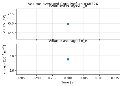
core_profiles_time_volume_averaged · shot 48224 Stalecore_profiles_profile_zeffcore_profiles_time_volume_averaged
time
source
core_profiles / time / volume_averaged · domain core_profiles · view model Panels
Volume-averaged core quantity panels on a shared time axis.
Thumbnail drawn from sample shot 48224, stale: renderer or style changed.
vaft.omas.plot_core_profiles_time_volume_averaged(ods) # from data
vaft.plot.core_profiles_time_volume_averaged(model) # from a PanelsShow source vaft/plot/renderers/panels.py, lines 912–925
@_panel_renderer(
domain="core_profiles",
subject="core_profiles",
view="time",
quantity="volume_averaged",
description="Volume-averaged core quantity panels on a shared time axis.",
ids=("core_profiles",),
required_paths=("core_profiles.time",),
)
def core_profiles_time_volume_averaged(
model: Panels, *, ax: Any = None, show: bool = False, **style: Any
) -> tuple[Figure, np.ndarray]:
"""Volume-averaged core quantity panels on a shared time axis."""
return render_panels(model, ax=ax, show=show, **style)| IDS | core_profiles |
|---|---|
| Required paths | core_profiles.time |
| Backends | matplotlib, plotly |
| Renderer | vaft.plot.renderers.panels.core_profiles_time_volume_averaged |
core_profiles_profile_zeff
profile
source
core_profiles / profile / zeff · domain core_profiles · view model Profile1D
Z_eff(rho) stored in a core_profiles slice, labelled measured, assumed, derived or inferred by its zeff_fit record; an unlabelled profile says so.
No thumbnail: no packaged sample carries the data this plot needs.
vaft.omas.plot_core_profiles_profile_zeff(ods) # from data
vaft.plot.core_profiles_profile_zeff(model) # from a Profile1DShow source vaft/plot/renderers/profiles.py, lines 307–325
@_profile_renderer(
domain="core_profiles", quantity="zeff",
subject="core_profiles",
description=(
"Z_eff(rho) stored in a core_profiles slice, labelled measured, assumed, derived or "
"inferred by its zeff_fit record; an unlabelled profile says so."
),
ids=("core_profiles",),
required_paths=(
"core_profiles.profiles_1d.{i}.zeff",
"core_profiles.profiles_1d.{i}.grid.rho_tor_norm",
),
optional_paths=("core_profiles.profiles_1d.{i}.zeff_fit.parameters",),
)
def core_profiles_profile_zeff(
model: Profile1D, *, ax: Axes | None = None, show: bool = False, **style: Any
) -> tuple[Figure, Axes]:
"""Stored Z_eff(rho), labelled by the origin its record states."""
return render_profile_1d(model, ax=ax, show=show, **style)| IDS | core_profiles |
|---|---|
| Required paths | core_profiles.profiles_1d.{i}.zeffcore_profiles.profiles_1d.{i}.grid.rho_tor_norm |
| Optional paths | core_profiles.profiles_1d.{i}.zeff_fit.parameters |
| Backends | matplotlib, plotly |
| Renderer | vaft.plot.renderers.profiles.core_profiles_profile_zeff |
Model subjects
vacuum [vacuum_field, null_field]
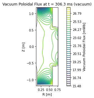
vacuum_field · shot 39915 Stale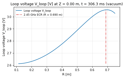
vacuum_field_midplane · shot 39915 Stalevacuum_field
field
source
vacuum / field · domain pf_active · view model Field2D
| The vacuum field of the coils and vessel at one instant: the flux, the poloidal field strength, the decay index, | E_phi | , the breakdown figure of merit, or the Lloyd margin, chosen with field=. |
Thumbnail drawn from sample shot 39915, stale: renderer or style changed.
vaft.omas.plot_vacuum_field(ods) # from data
vaft.plot.vacuum_field(model) # from a Field2DShow source vaft/plot/renderers/fields.py, lines 306–334
@_field_renderer(
domain="pf_active", quantity="",
subject="vacuum",
description="The vacuum field of the coils and vessel at one instant: the "
"flux, the poloidal field strength, the decay index, |E_phi|, "
"the breakdown figure of merit, or the Lloyd margin, chosen "
"with field=.",
# spectrometer_uv earns its place: with no time= the map is drawn at the
# breakdown onset, and that timing reads H-alpha alongside the plasma
# current. An adapter that loads only the declared IDSs would otherwise
# resolve a different instant than one that hands over the whole entry.
# barometry for the same reason, by a different route: field="lloyd_margin"
# reads the fill pressure, and discovery offers it only when a gauge is
# present, so an adapter loading only these IDSs would never offer it.
ids=("pf_active", "pf_passive", "wall", "tf", "equilibrium", "magnetics",
"spectrometer_uv", "barometry"),
required_paths=("pf_active.time", "pf_active.coil.{i}.current.data"),
optional_paths=(
"pf_passive.loop.{i}.element.{j}.geometry.outline.r",
"tf.b_field_tor_vacuum_r.data",
"wall.description_2d.{i}.limiter.unit.{j}.outline.r",
"barometry.gauge.{i}.pressure.data",
),
)
def vacuum_field(
model: Field2D, *, ax: Axes | None = None, show: bool = False, **style: Any
) -> tuple[Figure, Axes]:
"""One quantity of the coils' and vessel's vacuum field, at one instant."""
return render_field_2d(model, ax=ax, show=show, **style)| IDS | pf_active, pf_passive, wall, tf, equilibrium, magnetics, spectrometer_uv, barometry |
|---|---|
| Required paths | pf_active.timepf_active.coil.{i}.current.data |
| Optional paths | pf_passive.loop.{i}.element.{j}.geometry.outline.rtf.b_field_tor_vacuum_r.datawall.description_2d.{i}.limiter.unit.{j}.outline.rbarometry.gauge.{i}.pressure.data |
| Backends | matplotlib, plotly |
| Renderer | vaft.plot.renderers.fields.vacuum_field |
vacuum_field_midplane
field
source
vacuum / field / midplane · domain pf_active · view model LineSeries
One vacuum startup quantity along the Z = 0 row of the vacuum map – loop voltage, B_Z, the breakdown figure with its Ohmic and ECH-assisted thresholds, the Lloyd margin or the connection length – with the ECR radius, chosen with field=.
Thumbnail drawn from sample shot 39915, stale: renderer or style changed.
vaft.omas.plot_vacuum_field_midplane(ods) # from data
vaft.plot.vacuum_field_midplane(model) # from a LineSeriesShow source vaft/plot/renderers/lines.py, lines 1300–1326
@renderer(
domain="pf_active",
subject="vacuum",
view="field",
quantity="midplane",
model=LineSeries,
description="One vacuum startup quantity along the Z = 0 row of the vacuum map -- loop "
"voltage, B_Z, the breakdown figure with its Ohmic and ECH-assisted thresholds, "
"the Lloyd margin or the connection length -- with the ECR radius, chosen with field=.",
ids=("pf_active", "pf_passive", "wall", "tf", "equilibrium", "magnetics",
"spectrometer_uv", "barometry"),
required_paths=("pf_active.time", "pf_active.coil.{i}.current.data"),
optional_paths=(
"tf.b_field_tor_vacuum_r.data",
"wall.description_2d.{i}.limiter.unit.{j}.outline.r",
"barometry.gauge.{i}.pressure.data",
),
)
def vacuum_field_midplane(
model: LineSeries,
*,
ax: Axes | None = None,
show: bool = False,
**style: Any,
) -> tuple[Figure, Axes]:
"""One vacuum startup quantity along the midplane, at one instant."""
return render_line_series(model, ax=ax, show=show, **style)| IDS | pf_active, pf_passive, wall, tf, equilibrium, magnetics, spectrometer_uv, barometry |
|---|---|
| Required paths | pf_active.timepf_active.coil.{i}.current.data |
| Optional paths | tf.b_field_tor_vacuum_r.datawall.description_2d.{i}.limiter.unit.{j}.outline.rbarometry.gauge.{i}.pressure.data |
| Backends | matplotlib, plotly |
| Renderer | vaft.plot.renderers.lines.vacuum_field_midplane |
startup_proxies [startup]
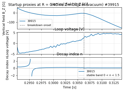
startup_proxies_time · shot 39915 Stalestartup_proxies_time
time
source
startup_proxies / time · domain pf_active · view model Panels
Vacuum B_Z, loop voltage and decay index at one (R, Z) point against time (rz=), from the OH-coil onset to the plasma-current peak, every entry overlaid with its breakdown onset marked (issue #888).
Thumbnail drawn from sample shot 39915, stale: renderer or style changed.
vaft.omas.plot_startup_proxies_time(ods) # from data
vaft.plot.startup_proxies_time(model) # from a PanelsShow source vaft/plot/renderers/panels.py, lines 1274–1292
@_panel_renderer(
domain="pf_active",
subject="startup_proxies",
view="time",
quantity="",
description=(
"Vacuum B_Z, loop voltage and decay index at one (R, Z) point against time "
"(rz=), from the OH-coil onset to the plasma-current peak, every entry overlaid "
"with its breakdown onset marked (issue #888)."
),
ids=("pf_active", "pf_passive", "wall", "tf", "equilibrium", "magnetics", "spectrometer_uv"),
required_paths=("pf_active.time", "pf_active.coil.{i}.current.data"),
optional_paths=("pf_passive.loop.{i}.element.{j}.geometry.outline.r",),
)
def startup_proxies_time(
model: Panels, *, ax: Any = None, show: bool = False, **style: Any
) -> tuple[Figure, np.ndarray]:
"""Vacuum startup proxies at one point against time, shots overlaid."""
return render_panels(model, ax=ax, show=show, **style)| IDS | pf_active, pf_passive, wall, tf, equilibrium, magnetics, spectrometer_uv |
|---|---|
| Required paths | pf_active.timepf_active.coil.{i}.current.data |
| Optional paths | pf_passive.loop.{i}.element.{j}.geometry.outline.r |
| Backends | matplotlib, plotly |
| Renderer | vaft.plot.renderers.panels.startup_proxies_time |
mhd_linear
mhd_linear_time_energy_perturbedmhd_linear_profile_b_field_perturbedmhd_linear_profile_chirikovmhd_linear_profile_displacementmhd_linear_profile_island_widthmhd_linear_profile_resonant_fluxmhd_linear_field_spectrummhd_linear_geometry_islandmhd_linear_spectrum_b_field_perturbedmhd_linear_overview_eigenfunctionmhd_linear_time_energy_perturbed
time
source
mhd_linear / time / energy_perturbed · domain mhd_linear · view model LineSeries
DCON perturbed potential energy against time, one trace per toroidal mode number; a negative value is an ideal-MHD unstable mode.
No thumbnail: no packaged sample carries the data this plot needs.
vaft.omas.plot_mhd_linear_time_energy_perturbed(ods) # from data
vaft.plot.mhd_linear_time_energy_perturbed(model) # from a LineSeriesShow source vaft/plot/renderers/lines.py, lines 1637–1657
@renderer(
domain="mhd_linear",
subject="mhd_linear",
view="time",
quantity="energy_perturbed",
model=LineSeries,
description=(
"DCON perturbed potential energy against time, one trace per toroidal "
"mode number; a negative value is an ideal-MHD unstable mode."
),
ids=("mhd_linear",),
required_paths=(
"mhd_linear.time_slice.{i}.toroidal_mode.{j}.n_tor",
"mhd_linear.time_slice.{i}.toroidal_mode.{j}.energy_perturbed",
),
)
def mhd_linear_time_energy_perturbed(
model: LineSeries, *, ax: Any = None, show: bool = False, **style: Any
) -> tuple[Figure, Any]:
"""Perturbed potential energy history per toroidal mode."""
return render_line_series(model, ax=ax, show=show, **style)| IDS | mhd_linear |
|---|---|
| Required paths | mhd_linear.time_slice.{i}.toroidal_mode.{j}.n_tormhd_linear.time_slice.{i}.toroidal_mode.{j}.energy_perturbed |
| Backends | matplotlib, plotly |
| Renderer | vaft.plot.renderers.lines.mhd_linear_time_energy_perturbed |
mhd_linear_profile_b_field_perturbed
profile
source
mhd_linear / profile / b_field_perturbed · domain mhd_linear · view model Profile1D
Normal perturbed field per poloidal harmonic against normalized flux, derived from the DCON eigenfunction as i(m - nq) xi.grad(psi).
No thumbnail: no packaged sample carries the data this plot needs.
vaft.omas.plot_mhd_linear_profile_b_field_perturbed(ods) # from data
vaft.plot.mhd_linear_profile_b_field_perturbed(model) # from a Profile1DShow source vaft/plot/renderers/profiles.py, lines 832–851
@_profile_renderer(
domain="mhd_linear", quantity="b_field_perturbed",
subject="mhd_linear",
description="Normal perturbed field per poloidal harmonic against normalized flux, "
"derived from the DCON eigenfunction as i(m - nq) xi.grad(psi).",
ids=("mhd_linear",),
required_paths=_MHD_LINEAR_EIGENFUNCTION_PATHS + (
"mhd_linear.time_slice.{i}.toroidal_mode.{j}.plasma.b_field_perturbed.coordinate1.real",
"mhd_linear.time_slice.{i}.toroidal_mode.{j}.plasma.b_field_perturbed.coordinate1.imaginary",
),
optional_paths=(
"mhd_linear.time_slice.{i}.toroidal_mode.{j}.energy_perturbed",
"mhd_linear.time_slice.{i}.toroidal_mode.{j}.m_pol_dominant",
),
)
def mhd_linear_profile_b_field_perturbed(
model: Profile1D, *, ax: Axes | None = None, show: bool = False, **style: Any
) -> tuple[Figure, Axes]:
"""Normal perturbed field per poloidal harmonic."""
return render_profile_1d(model, ax=ax, show=show, **style)| IDS | mhd_linear |
|---|---|
| Required paths | mhd_linear.time_slice.{i}.toroidal_mode.{j}.n_tormhd_linear.time_slice.{i}.toroidal_mode.{j}.plasma.grid.dim1mhd_linear.time_slice.{i}.toroidal_mode.{j}.plasma.grid.dim2mhd_linear.time_slice.{i}.toroidal_mode.{j}.plasma.b_field_perturbed.coordinate1.realmhd_linear.time_slice.{i}.toroidal_mode.{j}.plasma.b_field_perturbed.coordinate1.imaginary |
| Optional paths | mhd_linear.time_slice.{i}.toroidal_mode.{j}.energy_perturbedmhd_linear.time_slice.{i}.toroidal_mode.{j}.m_pol_dominant |
| Backends | matplotlib, plotly |
| Renderer | vaft.plot.renderers.profiles.mhd_linear_profile_b_field_perturbed |
mhd_linear_profile_chirikov
profile
source
mhd_linear / profile / chirikov · domain mhd_linear · view model Profile1D
Island-overlap parameter per rational surface against normalized poloidal flux, in GPEC's own surface definition, with the K = 1 criterion drawn; derived from the mapped perturbed flux.
No thumbnail: no packaged sample carries the data this plot needs.
vaft.omas.plot_mhd_linear_profile_chirikov(ods) # from data
vaft.plot.mhd_linear_profile_chirikov(model) # from a Profile1DShow source vaft/plot/renderers/profiles.py, lines 899–912
@_profile_renderer(
domain="mhd_linear", quantity="chirikov",
subject="mhd_linear",
description="Island-overlap parameter per rational surface against normalized "
"poloidal flux, in GPEC's own surface definition, with the K = 1 "
"criterion drawn; derived from the mapped perturbed flux.",
ids=("mhd_linear",),
required_paths=_GPEC_RESONANT_PATHS,
)
def mhd_linear_profile_chirikov(
model: Profile1D, *, ax: Axes | None = None, show: bool = False, **style: Any
) -> tuple[Figure, Axes]:
"""Island overlap per rational surface."""
return render_profile_1d(model, ax=ax, show=show, **style)| IDS | mhd_linear |
|---|---|
| Required paths | mhd_linear.time_slice.{i}.toroidal_mode.{j}.n_tormhd_linear.time_slice.{i}.toroidal_mode.{j}.plasma.grid.dim1mhd_linear.time_slice.{i}.toroidal_mode.{j}.plasma.grid.dim2mhd_linear.time_slice.{i}.toroidal_mode.{j}.plasma.b_field_perturbed.coordinate1.realmhd_linear.time_slice.{i}.toroidal_mode.{j}.plasma.b_field_perturbed.coordinate1.imaginarymhd_linear.code.parameters |
| Backends | matplotlib, plotly |
| Renderer | vaft.plot.renderers.profiles.mhd_linear_profile_chirikov |
mhd_linear_profile_displacement
profile
source
mhd_linear / profile / displacement · domain mhd_linear · view model Profile1D
DCON displacement eigenfunction against normalized flux, one trace per poloidal harmonic; amplitudes are normalized to the peak because DCON's eigenvector normalization is arbitrary.
No thumbnail: no packaged sample carries the data this plot needs.
vaft.omas.plot_mhd_linear_profile_displacement(ods) # from data
vaft.plot.mhd_linear_profile_displacement(model) # from a Profile1DShow source vaft/plot/renderers/profiles.py, lines 809–829
@_profile_renderer(
domain="mhd_linear", quantity="displacement",
subject="mhd_linear",
description="DCON displacement eigenfunction against normalized flux, one trace "
"per poloidal harmonic; amplitudes are normalized to the peak because "
"DCON's eigenvector normalization is arbitrary.",
ids=("mhd_linear",),
required_paths=_MHD_LINEAR_EIGENFUNCTION_PATHS + (
"mhd_linear.time_slice.{i}.toroidal_mode.{j}.plasma.displacement_perpendicular.real",
"mhd_linear.time_slice.{i}.toroidal_mode.{j}.plasma.displacement_perpendicular.imaginary",
),
optional_paths=(
"mhd_linear.time_slice.{i}.toroidal_mode.{j}.energy_perturbed",
"mhd_linear.time_slice.{i}.toroidal_mode.{j}.m_pol_dominant",
),
)
def mhd_linear_profile_displacement(
model: Profile1D, *, ax: Axes | None = None, show: bool = False, **style: Any
) -> tuple[Figure, Axes]:
"""DCON displacement eigenfunction per poloidal harmonic."""
return render_profile_1d(model, ax=ax, show=show, **style)| IDS | mhd_linear |
|---|---|
| Required paths | mhd_linear.time_slice.{i}.toroidal_mode.{j}.n_tormhd_linear.time_slice.{i}.toroidal_mode.{j}.plasma.grid.dim1mhd_linear.time_slice.{i}.toroidal_mode.{j}.plasma.grid.dim2mhd_linear.time_slice.{i}.toroidal_mode.{j}.plasma.displacement_perpendicular.realmhd_linear.time_slice.{i}.toroidal_mode.{j}.plasma.displacement_perpendicular.imaginary |
| Optional paths | mhd_linear.time_slice.{i}.toroidal_mode.{j}.energy_perturbedmhd_linear.time_slice.{i}.toroidal_mode.{j}.m_pol_dominant |
| Backends | matplotlib, plotly |
| Renderer | vaft.plot.renderers.profiles.mhd_linear_profile_displacement |
mhd_linear_profile_island_width
profile
source
mhd_linear / profile / island_width · domain mhd_linear · view model Profile1D
Saturated island width per rational surface against normalized poloidal flux, in psi_N as GPEC reports it, derived from the resonant flux.
No thumbnail: no packaged sample carries the data this plot needs.
vaft.omas.plot_mhd_linear_profile_island_width(ods) # from data
vaft.plot.mhd_linear_profile_island_width(model) # from a Profile1DShow source vaft/plot/renderers/profiles.py, lines 883–896
@_profile_renderer(
domain="mhd_linear", quantity="island_width",
subject="mhd_linear",
description="Saturated island width per rational surface against normalized "
"poloidal flux, in psi_N as GPEC reports it, derived from the "
"resonant flux.",
ids=("mhd_linear",),
required_paths=_GPEC_RESONANT_PATHS,
)
def mhd_linear_profile_island_width(
model: Profile1D, *, ax: Axes | None = None, show: bool = False, **style: Any
) -> tuple[Figure, Axes]:
"""Saturated island width per rational surface."""
return render_profile_1d(model, ax=ax, show=show, **style)| IDS | mhd_linear |
|---|---|
| Required paths | mhd_linear.time_slice.{i}.toroidal_mode.{j}.n_tormhd_linear.time_slice.{i}.toroidal_mode.{j}.plasma.grid.dim1mhd_linear.time_slice.{i}.toroidal_mode.{j}.plasma.grid.dim2mhd_linear.time_slice.{i}.toroidal_mode.{j}.plasma.b_field_perturbed.coordinate1.realmhd_linear.time_slice.{i}.toroidal_mode.{j}.plasma.b_field_perturbed.coordinate1.imaginarymhd_linear.code.parameters |
| Backends | matplotlib, plotly |
| Renderer | vaft.plot.renderers.profiles.mhd_linear_profile_island_width |
mhd_linear_profile_resonant_flux
profile
source
mhd_linear / profile / resonant_flux · domain mhd_linear · view model Profile1D
Pitch-resonant flux per rational surface against normalized poloidal flux, derived from the mapped perturbed flux by the jump across each singular surface rather than read from the IDS.
No thumbnail: no packaged sample carries the data this plot needs.
vaft.omas.plot_mhd_linear_profile_resonant_flux(ods) # from data
vaft.plot.mhd_linear_profile_resonant_flux(model) # from a Profile1DShow source vaft/plot/renderers/profiles.py, lines 867–880
@_profile_renderer(
domain="mhd_linear", quantity="resonant_flux",
subject="mhd_linear",
description="Pitch-resonant flux per rational surface against normalized poloidal "
"flux, derived from the mapped perturbed flux by the jump across each "
"singular surface rather than read from the IDS.",
ids=("mhd_linear",),
required_paths=_GPEC_RESONANT_PATHS,
)
def mhd_linear_profile_resonant_flux(
model: Profile1D, *, ax: Axes | None = None, show: bool = False, **style: Any
) -> tuple[Figure, Axes]:
"""Pitch-resonant flux per rational surface."""
return render_profile_1d(model, ax=ax, show=show, **style)| IDS | mhd_linear |
|---|---|
| Required paths | mhd_linear.time_slice.{i}.toroidal_mode.{j}.n_tormhd_linear.time_slice.{i}.toroidal_mode.{j}.plasma.grid.dim1mhd_linear.time_slice.{i}.toroidal_mode.{j}.plasma.grid.dim2mhd_linear.time_slice.{i}.toroidal_mode.{j}.plasma.b_field_perturbed.coordinate1.realmhd_linear.time_slice.{i}.toroidal_mode.{j}.plasma.b_field_perturbed.coordinate1.imaginarymhd_linear.code.parameters |
| Backends | matplotlib, plotly |
| Renderer | vaft.plot.renderers.profiles.mhd_linear_profile_resonant_flux |
mhd_linear_field_spectrum
field
source
mhd_linear / field / spectrum · domain mhd_linear · view model Field2D
Perturbed normal flux amplitude over the mapped (psi_N, m) grid: the radial label on the abscissa and the poloidal harmonic on the ordinate, which is why this map is not drawn to an equal aspect.
No thumbnail: no packaged sample carries the data this plot needs.
vaft.omas.plot_mhd_linear_field_spectrum(ods) # from data
vaft.plot.mhd_linear_field_spectrum(model) # from a Field2DShow source vaft/plot/renderers/fields.py, lines 445–467
@_field_renderer(
domain="mhd_linear", quantity="spectrum",
subject="mhd_linear",
description="Perturbed normal flux amplitude over the mapped (psi_N, m) grid: "
"the radial label on the abscissa and the poloidal harmonic on the "
"ordinate, which is why this map is not drawn to an equal aspect.",
ids=("mhd_linear",),
required_paths=(
"mhd_linear.time_slice.{i}.toroidal_mode.{j}.n_tor",
"mhd_linear.time_slice.{i}.toroidal_mode.{j}.plasma.grid.dim1",
"mhd_linear.time_slice.{i}.toroidal_mode.{j}.plasma.grid.dim2",
"mhd_linear.time_slice.{i}.toroidal_mode.{j}.plasma.b_field_perturbed.coordinate1.real",
"mhd_linear.time_slice.{i}.toroidal_mode.{j}.plasma.b_field_perturbed.coordinate1.imaginary",
),
optional_paths=(
"mhd_linear.time_slice.{i}.toroidal_mode.{j}.energy_perturbed",
),
)
def mhd_linear_field_spectrum(
model: Field2D, *, ax: Axes | None = None, show: bool = False, **style: Any
) -> tuple[Figure, Axes]:
"""Perturbed normal flux amplitude over the (psi_N, m) grid."""
return render_field_2d(model, ax=ax, show=show, **style)| IDS | mhd_linear |
|---|---|
| Required paths | mhd_linear.time_slice.{i}.toroidal_mode.{j}.n_tormhd_linear.time_slice.{i}.toroidal_mode.{j}.plasma.grid.dim1mhd_linear.time_slice.{i}.toroidal_mode.{j}.plasma.grid.dim2mhd_linear.time_slice.{i}.toroidal_mode.{j}.plasma.b_field_perturbed.coordinate1.realmhd_linear.time_slice.{i}.toroidal_mode.{j}.plasma.b_field_perturbed.coordinate1.imaginary |
| Optional paths | mhd_linear.time_slice.{i}.toroidal_mode.{j}.energy_perturbed |
| Backends | matplotlib, plotly |
| Renderer | vaft.plot.renderers.fields.mhd_linear_field_spectrum |
mhd_linear_geometry_island
geometry
source
mhd_linear / geometry / island · domain mhd_linear · view model GeometryLayers
Saturated island separatrices in the poloidal plane at one toroidal angle, derived from the mapped perturbed flux and drawn on the run's own flux-surface mesh; the island phase is GPEC's arg(I_res).
No thumbnail: no packaged sample carries the data this plot needs.
vaft.omas.plot_mhd_linear_geometry_island(ods) # from data
vaft.plot.mhd_linear_geometry_island(model) # from a GeometryLayersShow source vaft/plot/renderers/geometry.py, lines 631–657
@_geometry_renderer(
domain="mhd_linear", quantity="island",
subject="mhd_linear",
description="Saturated island separatrices in the poloidal plane at one toroidal "
"angle, derived from the mapped perturbed flux and drawn on the run's "
"own flux-surface mesh; the island phase is GPEC's arg(I_res).",
ids=("mhd_linear",),
required_paths=(
"mhd_linear.time_slice.{i}.toroidal_mode.{j}.n_tor",
"mhd_linear.time_slice.{i}.toroidal_mode.{j}.plasma.grid.dim1",
"mhd_linear.time_slice.{i}.toroidal_mode.{j}.plasma.grid.dim2",
"mhd_linear.time_slice.{i}.toroidal_mode.{j}.plasma.b_field_perturbed.coordinate1.real",
"mhd_linear.time_slice.{i}.toroidal_mode.{j}.plasma.b_field_perturbed.coordinate1.imaginary",
"mhd_linear.time_slice.{i}.toroidal_mode.{j}.plasma.coordinate_system.grid.dim1",
"mhd_linear.time_slice.{i}.toroidal_mode.{j}.plasma.coordinate_system.grid.dim2",
"mhd_linear.time_slice.{i}.toroidal_mode.{j}.plasma.coordinate_system.r",
"mhd_linear.time_slice.{i}.toroidal_mode.{j}.plasma.coordinate_system.z",
# The per-surface geometry and chi1 the resonant derivation needs;
# they have no IMAS slot, so the mapper records them here (D-12).
"mhd_linear.code.parameters",
),
)
def mhd_linear_geometry_island(
model: GeometryLayers, *, ax: Axes | None = None, show: bool = False, **style: Any
) -> tuple[Figure, Axes]:
"""Saturated island separatrices in the poloidal plane."""
return render_geometry_layers(model, ax=ax, show=show, **style)| IDS | mhd_linear |
|---|---|
| Required paths | mhd_linear.time_slice.{i}.toroidal_mode.{j}.n_tormhd_linear.time_slice.{i}.toroidal_mode.{j}.plasma.grid.dim1mhd_linear.time_slice.{i}.toroidal_mode.{j}.plasma.grid.dim2mhd_linear.time_slice.{i}.toroidal_mode.{j}.plasma.b_field_perturbed.coordinate1.realmhd_linear.time_slice.{i}.toroidal_mode.{j}.plasma.b_field_perturbed.coordinate1.imaginarymhd_linear.time_slice.{i}.toroidal_mode.{j}.plasma.coordinate_system.grid.dim1mhd_linear.time_slice.{i}.toroidal_mode.{j}.plasma.coordinate_system.grid.dim2mhd_linear.time_slice.{i}.toroidal_mode.{j}.plasma.coordinate_system.rmhd_linear.time_slice.{i}.toroidal_mode.{j}.plasma.coordinate_system.zmhd_linear.code.parameters |
| Backends | matplotlib |
| Renderer | vaft.plot.renderers.geometry.mhd_linear_geometry_island |
mhd_linear_spectrum_b_field_perturbed
spectrum
source
mhd_linear / spectrum / b_field_perturbed · domain mhd_linear · view model Profile1D
Perturbed normal flux amplitude against poloidal harmonic at one flux surface; the outermost mapped surface unless psi_n names another, and the title reports the surface actually drawn.
No thumbnail: no packaged sample carries the data this plot needs.
vaft.omas.plot_mhd_linear_spectrum_b_field_perturbed(ods) # from data
vaft.plot.mhd_linear_spectrum_b_field_perturbed(model) # from a Profile1DShow source vaft/plot/renderers/profiles.py, lines 924–940
@renderer(
domain="mhd_linear", subject="mhd_linear", view="spectrum",
quantity="b_field_perturbed", model=Profile1D,
description="Perturbed normal flux amplitude against poloidal harmonic at one "
"flux surface; the outermost mapped surface unless psi_n names "
"another, and the title reports the surface actually drawn.",
ids=("mhd_linear",),
required_paths=_MHD_LINEAR_SPECTRUM_PATHS,
optional_paths=(
"mhd_linear.time_slice.{i}.toroidal_mode.{j}.energy_perturbed",
),
)
def mhd_linear_spectrum_b_field_perturbed(
model: Profile1D, *, ax: Axes | None = None, show: bool = False, **style: Any
) -> tuple[Figure, Axes]:
"""Perturbed normal flux spectrum at one flux surface."""
return render_profile_1d(model, ax=ax, show=show, **style)| IDS | mhd_linear |
|---|---|
| Required paths | mhd_linear.time_slice.{i}.toroidal_mode.{j}.n_tormhd_linear.time_slice.{i}.toroidal_mode.{j}.plasma.grid.dim1mhd_linear.time_slice.{i}.toroidal_mode.{j}.plasma.grid.dim2mhd_linear.time_slice.{i}.toroidal_mode.{j}.plasma.b_field_perturbed.coordinate1.realmhd_linear.time_slice.{i}.toroidal_mode.{j}.plasma.b_field_perturbed.coordinate1.imaginary |
| Optional paths | mhd_linear.time_slice.{i}.toroidal_mode.{j}.energy_perturbed |
| Backends | matplotlib, plotly |
| Renderer | vaft.plot.renderers.profiles.mhd_linear_spectrum_b_field_perturbed |
mhd_linear_overview_eigenfunction
overview
source
mhd_linear / overview / eigenfunction · domain mhd_linear · view model Panels
The DCON eigenfunction of the least-stable mapped mode: displacement and normal perturbed field per poloidal harmonic.
No thumbnail: no packaged sample carries the data this plot needs.
vaft.omas.plot_mhd_linear_overview_eigenfunction(ods) # from data
vaft.plot.mhd_linear_overview_eigenfunction(model) # from a PanelsShow source vaft/plot/renderers/panels.py, lines 1486–1497
@_panel_renderer(
domain="mhd_linear", subject="mhd_linear", view="overview", quantity="eigenfunction",
description="The DCON eigenfunction of the least-stable mapped mode: displacement "
"and normal perturbed field per poloidal harmonic.",
ids=("mhd_linear",),
required_paths=("mhd_linear.time_slice.{i}.toroidal_mode.{j}.plasma.grid.dim1",),
)
def mhd_linear_overview_eigenfunction(
model: Panels, *, ax: Any = None, show: bool = False, **style: Any
) -> tuple[Figure, np.ndarray]:
"""Displacement and normal perturbed field of the least-stable mode."""
return render_panels(model, ax=ax, show=show, **style)| IDS | mhd_linear |
|---|---|
| Required paths | mhd_linear.time_slice.{i}.toroidal_mode.{j}.plasma.grid.dim1 |
| Backends | matplotlib, plotly |
| Renderer | vaft.plot.renderers.panels.mhd_linear_overview_eigenfunction |
ntms [tearing, delta_prime]
ntms_time_delta_prime
time
source
ntms / time / delta_prime · domain mhd_linear · view model LineSeries
Classical tearing index Delta-prime against time, one trace per rational surface; a positive value is a tearing-unstable surface. This is RDCON's and STRIDE's physical result, which has no slot under toroidal_mode and lives in ntms.
No thumbnail: no packaged sample carries the data this plot needs.
vaft.omas.plot_ntms_time_delta_prime(ods) # from data
vaft.plot.ntms_time_delta_prime(model) # from a LineSeriesShow source vaft/plot/renderers/lines.py, lines 1611–1634
@renderer(
domain="mhd_linear",
subject="ntms",
view="time",
quantity="delta_prime",
model=LineSeries,
description=(
"Classical tearing index Delta-prime against time, one trace per "
"rational surface; a positive value is a tearing-unstable surface. "
"This is RDCON's and STRIDE's physical result, which has no slot under "
"`toroidal_mode` and lives in `ntms`."
),
ids=("ntms",),
required_paths=(
"ntms.time_slice.{i}.mode.{j}.n_tor",
"ntms.time_slice.{i}.mode.{j}.m_pol",
"ntms.time_slice.{i}.mode.{j}.deltaw.{k}.value",
),
)
def ntms_time_delta_prime(
model: LineSeries, *, ax: Any = None, show: bool = False, **style: Any
) -> tuple[Figure, Any]:
"""Classical tearing index per rational surface, against time."""
return render_line_series(model, ax=ax, show=show, **style)| IDS | ntms |
|---|---|
| Required paths | ntms.time_slice.{i}.mode.{j}.n_torntms.time_slice.{i}.mode.{j}.m_polntms.time_slice.{i}.mode.{j}.deltaw.{k}.value |
| Backends | matplotlib, plotly |
| Renderer | vaft.plot.renderers.lines.ntms_time_delta_prime |
field_line_topology [connection_length, field_lines]
field_line_topology_field_connection_length
field
source
field_line_topology / field / connection_length · domain plasma_initiation · view model Field2D
Total connection length of every traced field line in one poloidal plane, on the rectangular grid they were launched from. The title names the toroidal angle the plane was traced at, because the IDS entry carries no toroidal coordinate and the map means nothing without it.
No thumbnail: no packaged sample carries the data this plot needs.
vaft.omas.plot_field_line_topology_field_connection_length(ods) # from data
vaft.plot.field_line_topology_field_connection_length(model) # from a Field2DShow source vaft/plot/renderers/fields.py, lines 470–496
@_field_renderer(
domain="plasma_initiation", quantity="connection_length",
subject="field_line_topology",
description="Total connection length of every traced field line in one "
"poloidal plane, on the rectangular grid they were launched "
"from. The title names the toroidal angle the plane was "
"traced at, because the IDS entry carries no toroidal "
"coordinate and the map means nothing without it.",
ids=("plasma_initiation",),
required_paths=(
"plasma_initiation.b_field_lines.{i}.grid.dim1",
"plasma_initiation.b_field_lines.{i}.grid.dim2",
"plasma_initiation.b_field_lines.{i}.starting_positions.r",
"plasma_initiation.b_field_lines.{i}.starting_positions.z",
"plasma_initiation.b_field_lines.{i}.lengths",
),
optional_paths=(
"plasma_initiation.b_field_lines.{i}.open_fraction",
"plasma_initiation.b_field_lines.{i}.time",
"plasma_initiation.code.parameters",
),
)
def field_line_topology_field_connection_length(
model: Field2D, *, ax: Axes | None = None, show: bool = False, **style: Any
) -> tuple[Figure, Axes]:
"""Connection length over one traced poloidal plane."""
return render_field_2d(model, ax=ax, show=show, **style)| IDS | plasma_initiation |
|---|---|
| Required paths | plasma_initiation.b_field_lines.{i}.grid.dim1plasma_initiation.b_field_lines.{i}.grid.dim2plasma_initiation.b_field_lines.{i}.starting_positions.rplasma_initiation.b_field_lines.{i}.starting_positions.zplasma_initiation.b_field_lines.{i}.lengths |
| Optional paths | plasma_initiation.b_field_lines.{i}.open_fractionplasma_initiation.b_field_lines.{i}.timeplasma_initiation.code.parameters |
| Backends | matplotlib, plotly |
| Renderer | vaft.plot.renderers.fields.field_line_topology_field_connection_length |
neoclassical [bootstrap_current]
neoclassical_profile_bootstrap_current
profile
source
neoclassical / profile / bootstrap_current · domain core_profiles · view model Profile1D
Bootstrap current density from each neoclassical model on one radial axis: the Sauter and Redl formulas against whatever solver result the ODS carries.
No thumbnail: shot 48224: ValueError: core_profiles slice 0 carries no zeff and no z_eff was supplied; the coefficients depend on it and this layer does not hold a machine default (CONTRIBUTING.md sends that to vest.yaml with a status).
vaft.omas.plot_neoclassical_profile_bootstrap_current(ods) # from data
vaft.plot.neoclassical_profile_bootstrap_current(model) # from a Profile1DShow source vaft/plot/renderers/profiles.py, lines 277–304
@_profile_renderer(
domain="core_profiles", quantity="bootstrap_current",
subject="neoclassical",
description=(
"Bootstrap current density from each neoclassical model on one radial axis: "
"the Sauter and Redl formulas against whatever solver result the ODS carries."
),
ids=("core_profiles", "equilibrium"),
required_paths=(
"equilibrium.time_slice.{i}.profiles_1d.rho_tor_norm",
"equilibrium.time_slice.{i}.profiles_1d.psi",
"equilibrium.time_slice.{i}.profiles_1d.q",
"equilibrium.time_slice.{i}.profiles_1d.f",
"core_profiles.profiles_1d.{i}.electrons.temperature",
# The electron density is required too, in either of its two spellings,
# which the recipe's own `available` predicate checks.
),
optional_paths=(
"equilibrium.time_slice.{i}.profiles_1d.trapped_fraction",
"core_profiles.profiles_1d.{i}.zeff",
"core_profiles.profiles_1d.{i}.j_bootstrap",
),
)
def neoclassical_profile_bootstrap_current(
model: Profile1D, *, ax: Axes | None = None, show: bool = False, **style: Any
) -> tuple[Figure, Axes]:
"""Bootstrap current density, one series per neoclassical model."""
return render_profile_1d(model, ax=ax, show=show, **style)| IDS | core_profiles, equilibrium |
|---|---|
| Required paths | equilibrium.time_slice.{i}.profiles_1d.rho_tor_normequilibrium.time_slice.{i}.profiles_1d.psiequilibrium.time_slice.{i}.profiles_1d.qequilibrium.time_slice.{i}.profiles_1d.fcore_profiles.profiles_1d.{i}.electrons.temperature |
| Optional paths | equilibrium.time_slice.{i}.profiles_1d.trapped_fractioncore_profiles.profiles_1d.{i}.zeffcore_profiles.profiles_1d.{i}.j_bootstrap |
| Backends | matplotlib, plotly |
| Renderer | vaft.plot.renderers.profiles.neoclassical_profile_bootstrap_current |
gyrokinetics [gyrokinetics_local, local_gyrokinetics, linear_spectrum]
gyrokinetics_profile_eigenfunctiongyrokinetics_spectrum_energy_fluxgyrokinetics_spectrum_frequencygyrokinetics_spectrum_growth_rategyrokinetics_spectrum_particle_fluxgyrokinetics_overviewgyrokinetics_profile_eigenfunction
profile
source
gyrokinetics / profile / eigenfunction · domain gyrokinetics_local · view model Profile1D
phi eigenfunction of the most unstable leading mode against the poloidal angle.
Interpretation
Shows the perturbed electrostatic potential of the leading eigenmode at the most unstable converged k_y of the run against the DD poloidal angle, in units of pi: its magnitude (emphasised), real and imaginary parts. The angle runs clockwise from the low-field-side midplane and extends beyond one poloidal turn along the field line (the ballooning angle), so the width of the envelope says how far the mode extends along the line: a narrow envelope centred on zero is a ballooning mode localised on the outboard side; a wide or lobed one reaches the inboard side. The amplitude is normalised as the eigenmode’s code.parameters states (for the CGYRO mapping, phi divided by its value at angle zero, final time), and the title names the k_y the eigenfunction belongs to.
Limitations
Only the first eigenmode of the k_y with the largest converged growth rate is drawn: further eigenmodes, other k_y, and the parallel vector potential and parallel magnetic field eigenfunctions are not. The phase convention is the mapping’s, so real and imaginary parts are comparable between runs only when both state the same normalisation; the magnitude is convention-free. The extended-angle range is what the solver stored, so an asymmetric range is the run’s, not a feature of the mode.
See Also
See Also
gyrokinetics_spectrum_growth_rate : the growth rate that picked this k_y.
No thumbnail: no packaged sample carries the data this plot needs.
vaft.omas.plot_gyrokinetics_profile_eigenfunction(ods) # from data
vaft.plot.gyrokinetics_profile_eigenfunction(model) # from a Profile1DShow source vaft/plot/renderers/gyrokinetics.py, lines 238–278
@renderer(
domain=_GK, subject="gyrokinetics", view="profile", quantity="eigenfunction",
model=Profile1D, ids=(_GK,),
description="phi eigenfunction of the most unstable leading mode against the poloidal angle.",
required_paths=(f"{_GK}.linear.wavevector.{{i}}.eigenmode.{{j}}.angle_pol",
f"{_GK}.linear.wavevector.{{i}}.eigenmode.{{j}}.fields.phi_potential_perturbed_norm"),
)
def gyrokinetics_profile_eigenfunction(
model: Profile1D, *, ax: Axes | None = None, show: bool = False, **style: Any
) -> tuple[Figure, Axes]:
"""Eigenfunction magnitude, real and imaginary parts.
Interpretation
--------------
Shows the perturbed electrostatic potential of the leading eigenmode at
the most unstable converged k_y of the run against the DD poloidal angle,
in units of pi: its magnitude (emphasised), real and imaginary parts. The
angle runs clockwise from the low-field-side midplane and extends beyond
one poloidal turn along the field line (the ballooning angle), so the
width of the envelope says how far the mode extends along the line: a
narrow envelope centred on zero is a ballooning mode localised on the
outboard side; a wide or lobed one reaches the inboard side. The
amplitude is normalised as the eigenmode's code.parameters states (for
the CGYRO mapping, phi divided by its value at angle zero, final time),
and the title names the k_y the eigenfunction belongs to.
Limitations
-----------
Only the first eigenmode of the k_y with the largest converged growth
rate is drawn: further eigenmodes, other k_y, and the parallel vector
potential and parallel magnetic field eigenfunctions are not. The phase
convention is the mapping's, so real and imaginary parts are comparable
between runs only when both state the same normalisation; the magnitude
is convention-free. The extended-angle range is what the solver stored,
so an asymmetric range is the run's, not a feature of the mode.
See Also
--------
gyrokinetics_spectrum_growth_rate : the growth rate that picked this k_y.
"""
return render_profile_1d(model, ax=ax, show=show, **style)| IDS | gyrokinetics_local |
|---|---|
| Required paths | gyrokinetics_local.linear.wavevector.{i}.eigenmode.{j}.angle_polgyrokinetics_local.linear.wavevector.{i}.eigenmode.{j}.fields.phi_potential_perturbed_norm |
| Backends | matplotlib, plotly |
| Renderer | vaft.plot.renderers.gyrokinetics.gyrokinetics_profile_eigenfunction |
gyrokinetics_spectrum_energy_flux
spectrum
source
gyrokinetics / spectrum / energy_flux · domain gyrokinetics_local · view model Profile1D
ky-resolved energy flux per species (quasilinear or nonlinear, as the IDS records).
Interpretation
Shows, for each species, the energy flux carried by each binormal
wavenumber – the k_x-summed fluxes_2d_k_x_sum of the IDS, summed over
the field components it holds (phi, A_parallel, B_parallel) – against k_y
rho_ref, in the IDS’s GKDB reference flux. The title says whether the IDS
records a quasilinear estimate (a TGLF saturation rule), a nonlinear
simulation, or a mix of both across the entries. It is read for which
scales carry the transport (the k_y of the peak), how the flux is shared
between electrons and ion species, and how two models’ spectra differ at
the same surface; the “unmatched” title note names what keeps two entries
from being one comparison. The horizontal range stops at 1.1 times the
last k_y at which any species still carries one per cent of its peak
flux, so a grid that runs into the electron scales does not flatten the
ion-scale structure; the series themselves keep every point.
Limitations
A quasilinear flux is the saturation model’s estimate, not a prediction of the gyrokinetic equations, and its amplitude depends on the rule; the overlay does not say which rule is closer to a nonlinear result. The flux is in the IDS’s reference units, not W/m2, and the field components are summed, so an electromagnetic contribution cannot be separated here. The k_x structure is summed away. The cut of the horizontal range is a display choice: a species whose flux never rises above one per cent of another’s peak is not what sets it.
See Also
See Also
gyrokinetics_spectrum_particle_flux : the particle flux per k_y. turbulent_transport_profile_energy_flux : the radial energy flux the models give core_transport.
No thumbnail: no packaged sample carries the data this plot needs.
vaft.omas.plot_gyrokinetics_spectrum_energy_flux(ods) # from data
vaft.plot.gyrokinetics_spectrum_energy_flux(model) # from a Profile1DShow source vaft/plot/renderers/gyrokinetics.py, lines 146–192
@_spectrum(
"energy_flux",
"ky-resolved energy flux per species (quasilinear or nonlinear, as the IDS records).",
(f"{_GK}.non_linear.binormal_wavevector_norm",),
(f"{_GK}.non_linear.fluxes_2d_k_x_sum.energy_phi_potential",
f"{_GK}.non_linear.fluxes_2d_k_x_sum.energy_a_field_parallel",
f"{_GK}.non_linear.fluxes_2d_k_x_sum.energy_b_field_parallel",
f"{_GK}.non_linear.quasi_linear"),
)
def gyrokinetics_spectrum_energy_flux(
model: Profile1D, *, ax: Axes | None = None, show: bool = False, **style: Any
) -> tuple[Figure, Axes]:
"""ky-resolved energy flux from gyrokinetics_local.
Interpretation
--------------
Shows, for each species, the energy flux carried by each binormal
wavenumber -- the k_x-summed ``fluxes_2d_k_x_sum`` of the IDS, summed over
the field components it holds (phi, A_parallel, B_parallel) -- against k_y
rho_ref, in the IDS's GKDB reference flux. The title says whether the IDS
records a quasilinear estimate (a TGLF saturation rule), a nonlinear
simulation, or a mix of both across the entries. It is read for which
scales carry the transport (the k_y of the peak), how the flux is shared
between electrons and ion species, and how two models' spectra differ at
the same surface; the "unmatched" title note names what keeps two entries
from being one comparison. The horizontal range stops at 1.1 times the
last k_y at which any species still carries one per cent of its peak
flux, so a grid that runs into the electron scales does not flatten the
ion-scale structure; the series themselves keep every point.
Limitations
-----------
A quasilinear flux is the saturation model's estimate, not a prediction
of the gyrokinetic equations, and its amplitude depends on the rule;
the overlay does not say which rule is closer to a nonlinear result. The
flux is in the IDS's reference units, not W/m2, and the field components
are summed, so an electromagnetic contribution cannot be separated here.
The k_x structure is summed away. The cut of the horizontal range is a
display choice: a species whose flux never rises above one per cent of
another's peak is not what sets it.
See Also
--------
gyrokinetics_spectrum_particle_flux : the particle flux per k_y.
turbulent_transport_profile_energy_flux : the radial energy flux the models give core_transport.
"""
return render_profile_1d(model, ax=ax, show=show, **style)| IDS | gyrokinetics_local |
|---|---|
| Required paths | gyrokinetics_local.non_linear.binormal_wavevector_norm |
| Optional paths | gyrokinetics_local.non_linear.fluxes_2d_k_x_sum.energy_phi_potentialgyrokinetics_local.non_linear.fluxes_2d_k_x_sum.energy_a_field_parallelgyrokinetics_local.non_linear.fluxes_2d_k_x_sum.energy_b_field_parallelgyrokinetics_local.non_linear.quasi_linear |
| Backends | matplotlib, plotly |
| Renderer | vaft.plot.renderers.gyrokinetics.gyrokinetics_spectrum_energy_flux |
gyrokinetics_spectrum_frequency
spectrum
source
gyrokinetics / spectrum / frequency · domain gyrokinetics_local · view model Profile1D
Linear real frequency against k_y with each IDS's recorded sign convention.
Interpretation
Shows the real frequency of each eigenmode against the binormal wavenumber, in the IDS’s GKDB normalisation (k_y rho_ref against omega R0 / v_th,ref), with the same leading-mode solid, further-mode dotted layout as the growth-rate spectrum. The sign of the frequency tells the propagation direction, so the vertical label repeats the convention the IDS records in its code.parameters: “ion dia. < 0” when every entry stores the ion-diamagnetic-negative convention, “sign convention not recorded” when none does, and “sign conventions differ” when the entries disagree. A change of sign along k_y marks a change of the dominant branch; the growth-rate spectrum says which of them is unstable. Overlaid entries carry the same “unmatched” title note as the growth-rate spectrum.
Limitations
The sign is drawn as stored and never flipped: entries recorded under different conventions are labelled as differing, not reconciled, so their curves must not be compared by sign. The frequency of an unconverged initial-value run is its last-step value and is left out by default. A propagation direction does not by itself identify the instability branch.
See Also
See Also
gyrokinetics_spectrum_growth_rate : the growth rate of the same modes.
No thumbnail: no packaged sample carries the data this plot needs.
vaft.omas.plot_gyrokinetics_spectrum_frequency(ods) # from data
vaft.plot.gyrokinetics_spectrum_frequency(model) # from a Profile1DShow source vaft/plot/renderers/gyrokinetics.py, lines 99–143
@_spectrum(
"frequency",
"Linear real frequency against k_y with each IDS's recorded sign convention.",
(f"{_GK}.linear.wavevector.{{i}}.binormal_wavevector_norm",
f"{_GK}.linear.wavevector.{{i}}.eigenmode.{{j}}.frequency_norm"),
(f"{_GK}.code.parameters",),
)
def gyrokinetics_spectrum_frequency(
model: Profile1D, *, ax: Axes | None = None, show: bool = False, **style: Any
) -> tuple[Figure, Axes]:
"""Linear frequency spectrum from gyrokinetics_local.
Interpretation
--------------
Shows the real frequency of each eigenmode against the binormal
wavenumber, in the IDS's GKDB normalisation (k_y rho_ref against omega R0
/ v_th,ref), with the same leading-mode solid, further-mode dotted layout
as the growth-rate spectrum. The sign of the frequency tells the
propagation direction, so the vertical label repeats the convention the
IDS records in its code.parameters: "ion dia. < 0" when every entry
stores the ion-diamagnetic-negative convention, "sign convention not
recorded" when none does, and "sign conventions differ" when the entries
disagree. A change of sign along k_y marks a change of the dominant
branch; the growth-rate spectrum says which of them is unstable. Overlaid
entries carry the same "unmatched" title note as the growth-rate spectrum.
Options
-------
``include_unconverged=`` (default False) also draws initial-value
eigenmodes that reached no growth-rate tolerance.
Limitations
-----------
The sign is drawn as stored and never flipped: entries recorded under
different conventions are labelled as differing, not reconciled, so their
curves must not be compared by sign. The frequency of an unconverged
initial-value run is its last-step value and is left out by default. A
propagation direction does not by itself identify the instability
branch.
See Also
--------
gyrokinetics_spectrum_growth_rate : the growth rate of the same modes.
"""
return render_profile_1d(model, ax=ax, show=show, **style)| IDS | gyrokinetics_local |
|---|---|
| Required paths | gyrokinetics_local.linear.wavevector.{i}.binormal_wavevector_normgyrokinetics_local.linear.wavevector.{i}.eigenmode.{j}.frequency_norm |
| Optional paths | gyrokinetics_local.code.parameters |
| Backends | matplotlib, plotly |
| Renderer | vaft.plot.renderers.gyrokinetics.gyrokinetics_spectrum_frequency |
gyrokinetics_spectrum_growth_rate
spectrum
source
gyrokinetics / spectrum / growth_rate · domain gyrokinetics_local · view model Profile1D
Linear growth rate against k_y (GKDB normalisation), every eigenmode, entries overlaid.
Interpretation
Shows the linear growth rate of each eigenmode of one local flux-tube calculation against the binormal wavenumber, in the normalisation the IDS records (GKDB: lengths by R0, velocities by v_th,ref = sqrt(2 Te / mD), so the axes read k_y rho_ref and gamma R0 / v_th,ref). It is read for which k_y range is unstable, where the growth rate peaks, and how the spectrum of one run compares with another’s at the same surface: a scan merged from single-k_y runs or a quasilinear model’s spectrum drawn over a gyrokinetic one. The leading eigenmode of each entry is a solid line; further eigenmodes, where the solver writes them, are dotted and numbered. A k_y at which a mode is absent is a gap, never a zero. When several entries are overlaid, the title says “unmatched” and names what differs between them – surface, q, shear, species charges, field model, frequency sign convention or normalisation – read from each IDS’s own metadata, so an overlay that is not one comparison is marked, not silently drawn.
Limitations
The values are in the IDS’s GKDB normalisation, not the solver’s native units (CGYRO’s c_s / a, say); a native-unit spectrum is a different quantity and lives in the validation layer. Unconverged modes are not drawn, so a gap may be an unfinished run rather than a stable k_y. The mismatch mark compares metadata, not physics: two entries that agree on every listed key can still differ in resolution or collision model. The plot infers no instability branch (ITG, TEM, ETG, KBM, MTM) from the curve.
See Also
See Also
gyrokinetics_spectrum_frequency : the real frequency of the same modes. gyrokinetics_overview : the spectra with the run’s flux, eigenfunction and local state.
No thumbnail: no packaged sample carries the data this plot needs.
vaft.omas.plot_gyrokinetics_spectrum_growth_rate(ods) # from data
vaft.plot.gyrokinetics_spectrum_growth_rate(model) # from a Profile1DShow source vaft/plot/renderers/gyrokinetics.py, lines 44–96
@_spectrum(
"growth_rate",
"Linear growth rate against k_y (GKDB normalisation), every eigenmode, entries overlaid.",
(f"{_GK}.linear.wavevector.{{i}}.binormal_wavevector_norm",
f"{_GK}.linear.wavevector.{{i}}.eigenmode.{{j}}.growth_rate_norm"),
)
def gyrokinetics_spectrum_growth_rate(
model: Profile1D, *, ax: Axes | None = None, show: bool = False, **style: Any
) -> tuple[Figure, Axes]:
"""Linear growth rate spectrum from gyrokinetics_local.
Interpretation
--------------
Shows the linear growth rate of each eigenmode of one local flux-tube
calculation against the binormal wavenumber, in the normalisation the IDS
records (GKDB: lengths by R0, velocities by v_th,ref = sqrt(2 Te / mD), so
the axes read k_y rho_ref and gamma R0 / v_th,ref). It is read for which
k_y range is unstable, where the growth rate peaks, and how the spectrum
of one run compares with another's at the same surface: a scan merged
from single-k_y runs or a quasilinear model's spectrum drawn over a
gyrokinetic one. The leading eigenmode of each entry is a solid line;
further eigenmodes, where the solver writes them, are dotted and
numbered. A k_y at which a mode is absent is a gap, never a zero. When
several entries are overlaid, the title says "unmatched" and names what
differs between them -- surface, q, shear, species charges, field model,
frequency sign convention or normalisation -- read from each IDS's own
metadata, so an overlay that is not one comparison is marked, not
silently drawn.
Options
-------
``include_unconverged=`` (default False) also draws initial-value
eigenmodes that reached no growth-rate tolerance; by default they are left
out, because a run stopped at its time limit holds a last-step value, not
an eigenvalue.
Limitations
-----------
The values are in the IDS's GKDB normalisation, not the solver's native
units (CGYRO's c_s / a, say); a native-unit spectrum is a different
quantity and lives in the validation layer. Unconverged modes are not
drawn, so a gap may be an unfinished run rather than a stable k_y. The
mismatch mark compares metadata, not physics: two entries that agree on
every listed key can still differ in resolution or collision model. The
plot infers no instability branch (ITG, TEM, ETG, KBM, MTM) from the
curve.
See Also
--------
gyrokinetics_spectrum_frequency : the real frequency of the same modes.
gyrokinetics_overview : the spectra with the run's flux, eigenfunction and local state.
"""
return render_profile_1d(model, ax=ax, show=show, **style)| IDS | gyrokinetics_local |
|---|---|
| Required paths | gyrokinetics_local.linear.wavevector.{i}.binormal_wavevector_normgyrokinetics_local.linear.wavevector.{i}.eigenmode.{j}.growth_rate_norm |
| Backends | matplotlib, plotly |
| Renderer | vaft.plot.renderers.gyrokinetics.gyrokinetics_spectrum_growth_rate |
gyrokinetics_spectrum_particle_flux
spectrum
source
gyrokinetics / spectrum / particle_flux · domain gyrokinetics_local · view model Profile1D
ky-resolved particle flux per species.
Interpretation
Shows, for each species, the particle flux carried by each binormal
wavenumber – the k_x-summed fluxes_2d_k_x_sum of the IDS, summed over
the field components it holds – against k_y rho_ref, in the IDS’s GKDB
reference flux, with the quasilinear or nonlinear origin in the title. It
is read for the sign of the particle flux per scale (an inward, pinch-like
contribution at some k_y is as physical as an outward one), for the
scales that carry it, and for the species balance that ambipolarity
imposes on the sum. Overlaid entries carry the “unmatched” title note of
the other gyrokinetic spectra. The horizontal range stops where every
species’ flux has fallen below one per cent of its peak magnitude; the
series keep every point.
Limitations
A quasilinear flux is the saturation model’s estimate; its amplitude is the rule’s. The values are reference-normalised, not m-2 s-1, and the field components are summed. The k_x structure is summed away. The display cut of the horizontal range follows the peak magnitude, so a small flux of one species is not what sets it.
See Also
See Also
gyrokinetics_spectrum_energy_flux : the energy flux per k_y. turbulent_transport_profile_particle_flux : the radial particle flux the models give core_transport.
No thumbnail: no packaged sample carries the data this plot needs.
vaft.omas.plot_gyrokinetics_spectrum_particle_flux(ods) # from data
vaft.plot.gyrokinetics_spectrum_particle_flux(model) # from a Profile1DShow source vaft/plot/renderers/gyrokinetics.py, lines 195–235
@_spectrum(
"particle_flux",
"ky-resolved particle flux per species.",
(f"{_GK}.non_linear.binormal_wavevector_norm",),
(f"{_GK}.non_linear.fluxes_2d_k_x_sum.particles_phi_potential",
f"{_GK}.non_linear.fluxes_2d_k_x_sum.particles_a_field_parallel",
f"{_GK}.non_linear.fluxes_2d_k_x_sum.particles_b_field_parallel"),
)
def gyrokinetics_spectrum_particle_flux(
model: Profile1D, *, ax: Axes | None = None, show: bool = False, **style: Any
) -> tuple[Figure, Axes]:
"""ky-resolved particle flux from gyrokinetics_local.
Interpretation
--------------
Shows, for each species, the particle flux carried by each binormal
wavenumber -- the k_x-summed ``fluxes_2d_k_x_sum`` of the IDS, summed over
the field components it holds -- against k_y rho_ref, in the IDS's GKDB
reference flux, with the quasilinear or nonlinear origin in the title. It
is read for the sign of the particle flux per scale (an inward, pinch-like
contribution at some k_y is as physical as an outward one), for the
scales that carry it, and for the species balance that ambipolarity
imposes on the sum. Overlaid entries carry the "unmatched" title note of
the other gyrokinetic spectra. The horizontal range stops where every
species' flux has fallen below one per cent of its peak magnitude; the
series keep every point.
Limitations
-----------
A quasilinear flux is the saturation model's estimate; its amplitude is
the rule's. The values are reference-normalised, not m-2 s-1, and the
field components are summed. The k_x structure is summed away. The
display cut of the horizontal range follows the peak magnitude, so a
small flux of one species is not what sets it.
See Also
--------
gyrokinetics_spectrum_energy_flux : the energy flux per k_y.
turbulent_transport_profile_particle_flux : the radial particle flux the models give core_transport.
"""
return render_profile_1d(model, ax=ax, show=show, **style)| IDS | gyrokinetics_local |
|---|---|
| Required paths | gyrokinetics_local.non_linear.binormal_wavevector_norm |
| Optional paths | gyrokinetics_local.non_linear.fluxes_2d_k_x_sum.particles_phi_potentialgyrokinetics_local.non_linear.fluxes_2d_k_x_sum.particles_a_field_parallelgyrokinetics_local.non_linear.fluxes_2d_k_x_sum.particles_b_field_parallel |
| Backends | matplotlib, plotly |
| Renderer | vaft.plot.renderers.gyrokinetics.gyrokinetics_spectrum_particle_flux |
gyrokinetics_overview
overview
source
gyrokinetics / overview · domain gyrokinetics_local · view model Panels
One local gyrokinetic run: spectra, flux, eigenfunction and local state.
Interpretation
One figure for one local run: the growth-rate and frequency spectra, the k_y-resolved energy flux and the leading eigenfunction, each present only when the IDS carries it, beside a text column with the local state the run was given – r/R0, q, shear, elongation, the reference beta, each species’ normalised density and temperature gradients, the code and its commit, and the locality verdict when one was recorded. It is read as the first look at a run: whether it is unstable, at which scale, in which direction the modes propagate, how much flux the model attributes to them, and what plasma state produced all that. The suptitle names the code, its saturation rule and field model, and the surface.
Limitations
A missing quantity drops its panel without a note, so a figure with fewer panels says that the IDS lacks them, not that they were computed and empty. The members carry the readings and limitations of their own plots (GKDB normalisation, converged modes only, leading eigenmode only, the flux panel’s display range). One run per figure: comparisons are made by overlaying entries on the individual spectra.
See Also
See Also
gyrokinetics_spectrum_growth_rate : the growth-rate panel, with entries overlaid. gyrokinetics_profile_eigenfunction : the eigenfunction panel.
No thumbnail: no packaged sample carries the data this plot needs.
vaft.omas.plot_gyrokinetics_overview(ods) # from data
vaft.plot.gyrokinetics_overview(model) # from a PanelsShow source vaft/plot/renderers/gyrokinetics.py, lines 281–324
@renderer(
domain=_GK, subject="gyrokinetics", view="overview", model=Panels, ids=(_GK,),
description="One local gyrokinetic run: spectra, flux, eigenfunction and local state.",
required_paths=(f"{_GK}.flux_surface.r_minor_norm",),
)
def gyrokinetics_overview(
model: Panels, *, ax: Any = None, show: bool = False, **style: Any
) -> tuple[Figure, Any]:
"""Composite of the gyrokinetic panels the run supports.
Interpretation
--------------
One figure for one local run: the growth-rate and frequency spectra,
the k_y-resolved energy flux and the leading eigenfunction, each present
only when the IDS carries it, beside a text column with the local state
the run was given -- r/R0, q, shear, elongation, the reference beta,
each species' normalised density and temperature gradients, the code and
its commit, and the locality verdict when one was recorded. It is read
as the first look at a run: whether it is unstable, at which scale, in
which direction the modes propagate, how much flux the model attributes
to them, and what plasma state produced all that. The suptitle names the
code, its saturation rule and field model, and the surface.
Options
-------
``include_unconverged=`` (default False) also draws, in the two linear
spectra, the initial-value eigenmodes that reached no growth-rate
tolerance. ``title=`` replaces the suptitle.
Limitations
-----------
A missing quantity drops its panel without a note, so a figure with fewer
panels says that the IDS lacks them, not that they were computed and
empty. The members carry the readings and limitations of their own plots
(GKDB normalisation, converged modes only, leading eigenmode only, the
flux panel's display range). One run per figure: comparisons are made by
overlaying entries on the individual spectra.
See Also
--------
gyrokinetics_spectrum_growth_rate : the growth-rate panel, with entries overlaid.
gyrokinetics_profile_eigenfunction : the eigenfunction panel.
"""
return render_panels(model, ax=ax, show=show, **style)| IDS | gyrokinetics_local |
|---|---|
| Required paths | gyrokinetics_local.flux_surface.r_minor_norm |
| Backends | matplotlib, plotly |
| Renderer | vaft.plot.renderers.gyrokinetics.gyrokinetics_overview |
turbulent_transport [anomalous_transport, turbulent_flux]
turbulent_transport_profile_energy_fluxturbulent_transport_profile_particle_fluxturbulent_transport_overviewturbulent_transport_profile_energy_flux
profile
source
turbulent_transport / profile / energy_flux · domain core_transport · view model Profile1D
Turbulent electron and ion energy flux against rho_tor_norm.
Interpretation
Shows the radial profile of the turbulent energy flux that each anomalous core_transport model (identifier index 6: a TGLF saturation rule, a gyrokinetic surrogate, a nonlinear run) gives at its flux-surface grid, against the normalised toroidal flux coordinate, in W/m2. Each model has one colour; its electron flux is solid and the sum of its ion species’ fluxes dashed, and overlaid entries name the model after their label. It is read for where the transport is predicted to sit radially, for the electron-to-ion share, and for how far the models of one family (several saturation rules, say) disagree on the same profile.
Limitations
The flux is each model’s output on the state it was given, not a measurement, and the plot does not set it against a power balance or an experimental flux. Only anomalous models are drawn: neoclassical or total-transport models in the same IDS are not. An ion species whose flux is not stored on the grid of the electron flux is left out of the ion sum without a note. A radially sparse grid (a handful of surfaces) is drawn as stored, with no interpolation between them.
See Also
See Also
turbulent_transport_profile_particle_flux : the particle flux of the same models. gyrokinetics_spectrum_energy_flux : the k_y-resolved flux behind one surface’s value.
No thumbnail: no packaged sample carries the data this plot needs.
vaft.omas.plot_turbulent_transport_profile_energy_flux(ods) # from data
vaft.plot.turbulent_transport_profile_energy_flux(model) # from a Profile1DShow source vaft/plot/renderers/gyrokinetics.py, lines 340–378
@_transport("energy_flux", "Turbulent electron and ion energy flux against rho_tor_norm.")
def turbulent_transport_profile_energy_flux(
model: Profile1D, *, ax: Axes | None = None, show: bool = False, **style: Any
) -> tuple[Figure, Axes]:
"""Turbulent energy flux profiles, one pair per anomalous model.
Interpretation
--------------
Shows the radial profile of the turbulent energy flux that each anomalous
core_transport model (identifier index 6: a TGLF saturation rule, a
gyrokinetic surrogate, a nonlinear run) gives at its flux-surface grid,
against the normalised toroidal flux coordinate, in W/m2. Each model has
one colour; its electron flux is solid and the sum of its ion species'
fluxes dashed, and overlaid entries name the model after their label. It
is read for where the transport is predicted to sit radially, for the
electron-to-ion share, and for how far the models of one family (several
saturation rules, say) disagree on the same profile.
Options
-------
``time=`` selects, per model, the stored profiles_1d slice nearest the
requested time; without it the first slice is drawn.
Limitations
-----------
The flux is each model's output on the state it was given, not a
measurement, and the plot does not set it against a power balance or an
experimental flux. Only anomalous models are drawn: neoclassical or
total-transport models in the same IDS are not. An ion species whose flux
is not stored on the grid of the electron flux is left out of the ion sum
without a note. A radially sparse grid (a handful of surfaces) is drawn
as stored, with no interpolation between them.
See Also
--------
turbulent_transport_profile_particle_flux : the particle flux of the same models.
gyrokinetics_spectrum_energy_flux : the k_y-resolved flux behind one surface's value.
"""
return render_profile_1d(model, ax=ax, show=show, **style)| IDS | core_transport |
|---|---|
| Required paths | core_transport.model.{i}.identifier.indexcore_transport.model.{i}.profiles_1d.{j}.grid_flux.rho_tor_normcore_transport.model.{i}.profiles_1d.{j}.electrons.energy.flux |
| Backends | matplotlib, plotly |
| Renderer | vaft.plot.renderers.gyrokinetics.turbulent_transport_profile_energy_flux |
turbulent_transport_profile_particle_flux
profile
source
turbulent_transport / profile / particle_flux · domain core_transport · view model Profile1D
Turbulent electron and ion particle flux against rho_tor_norm.
Interpretation
Shows the radial profile of the turbulent particle flux that each anomalous core_transport model (identifier index 6) gives at its flux-surface grid, against the normalised toroidal flux coordinate, in particles per m2 per s, with the same colour-per-model, electrons solid and ions dashed layout as the energy-flux profile. It is read for the sign of the predicted particle flux along the radius (an inward, pinch-like region as much as an outward one), for the species balance, and for the spread between the models of one family.
Limitations
The flux is each model’s output, not a measurement, and no particle source or density evolution is set against it here. Only anomalous models are drawn. An ion species stored off the electron grid is left out of the ion sum without a note, and a sparse grid is drawn as stored.
See Also
See Also
turbulent_transport_profile_energy_flux : the energy flux of the same models. gyrokinetics_spectrum_particle_flux : the k_y-resolved flux behind one surface’s value.
No thumbnail: no packaged sample carries the data this plot needs.
vaft.omas.plot_turbulent_transport_profile_particle_flux(ods) # from data
vaft.plot.turbulent_transport_profile_particle_flux(model) # from a Profile1DShow source vaft/plot/renderers/gyrokinetics.py, lines 381–415
@_transport("particle_flux", "Turbulent electron and ion particle flux against rho_tor_norm.")
def turbulent_transport_profile_particle_flux(
model: Profile1D, *, ax: Axes | None = None, show: bool = False, **style: Any
) -> tuple[Figure, Axes]:
"""Turbulent particle flux profiles, one pair per anomalous model.
Interpretation
--------------
Shows the radial profile of the turbulent particle flux that each
anomalous core_transport model (identifier index 6) gives at its
flux-surface grid, against the normalised toroidal flux coordinate, in
particles per m2 per s, with the same colour-per-model, electrons solid
and ions dashed layout as the energy-flux profile. It is read for the
sign of the predicted particle flux along the radius (an inward,
pinch-like region as much as an outward one), for the species balance,
and for the spread between the models of one family.
Options
-------
``time=`` selects, per model, the stored profiles_1d slice nearest the
requested time; without it the first slice is drawn.
Limitations
-----------
The flux is each model's output, not a measurement, and no particle
source or density evolution is set against it here. Only anomalous
models are drawn. An ion species stored off the electron grid is left out
of the ion sum without a note, and a sparse grid is drawn as stored.
See Also
--------
turbulent_transport_profile_energy_flux : the energy flux of the same models.
gyrokinetics_spectrum_particle_flux : the k_y-resolved flux behind one surface's value.
"""
return render_profile_1d(model, ax=ax, show=show, **style)| IDS | core_transport |
|---|---|
| Required paths | core_transport.model.{i}.identifier.indexcore_transport.model.{i}.profiles_1d.{j}.grid_flux.rho_tor_normcore_transport.model.{i}.profiles_1d.{j}.electrons.particles.flux |
| Backends | matplotlib, plotly |
| Renderer | vaft.plot.renderers.gyrokinetics.turbulent_transport_profile_particle_flux |
turbulent_transport_overview
overview
source
turbulent_transport / overview · domain core_transport · view model Panels
Turbulent energy and particle flux profiles side by side.
Interpretation
The turbulent energy-flux and particle-flux profiles of the anomalous core_transport models side by side on one radial axis, so the scales that carry energy and the scales that carry particles can be read against each other for every model at once: where both peak, whether the particle flux changes sign where the energy flux does not, and whether the models of one family spread more in one channel than in the other. Colours and line styles are those of the member profiles (one colour per model, electrons solid, ions dashed).
Limitations
The members’ limitations apply: model outputs rather than measurements, anomalous models only, ion sums over the species stored on the electron grid, no interpolation between sparse surfaces. The two panels share the radial axis, not a flux scale.
See Also
See Also
turbulent_transport_profile_energy_flux : the left panel on its own. turbulent_transport_profile_particle_flux : the right panel on its own.
No thumbnail: no packaged sample carries the data this plot needs.
vaft.omas.plot_turbulent_transport_overview(ods) # from data
vaft.plot.turbulent_transport_overview(model) # from a PanelsShow source vaft/plot/renderers/gyrokinetics.py, lines 418–456
@renderer(
domain="core_transport", subject="turbulent_transport", view="overview", model=Panels,
ids=("core_transport",), description="Turbulent energy and particle flux profiles side by side.",
required_paths=("core_transport.model.{i}.identifier.index",),
)
def turbulent_transport_overview(
model: Panels, *, ax: Any = None, show: bool = False, **style: Any
) -> tuple[Figure, Any]:
"""Composite of the turbulent flux profiles.
Interpretation
--------------
The turbulent energy-flux and particle-flux profiles of the anomalous
core_transport models side by side on one radial axis, so the scales that
carry energy and the scales that carry particles can be read against each
other for every model at once: where both peak, whether the particle flux
changes sign where the energy flux does not, and whether the models of one
family spread more in one channel than in the other. Colours and line
styles are those of the member profiles (one colour per model, electrons
solid, ions dashed).
Options
-------
``time=`` selects, per model, the stored profiles_1d slice nearest the
requested time in both panels.
Limitations
-----------
The members' limitations apply: model outputs rather than measurements,
anomalous models only, ion sums over the species stored on the electron
grid, no interpolation between sparse surfaces. The two panels share the
radial axis, not a flux scale.
See Also
--------
turbulent_transport_profile_energy_flux : the left panel on its own.
turbulent_transport_profile_particle_flux : the right panel on its own.
"""
return render_panels(model, ax=ax, show=show, **style)| IDS | core_transport |
|---|---|
| Required paths | core_transport.model.{i}.identifier.index |
| Backends | matplotlib, plotly |
| Renderer | vaft.plot.renderers.gyrokinetics.turbulent_transport_overview |
impurity [impurities]
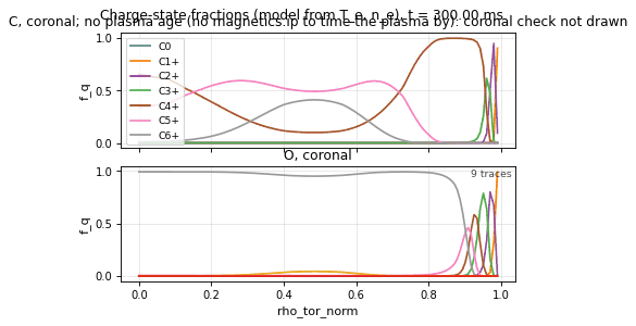
impurity_profile_charge_state_fraction · shot 48224 Stale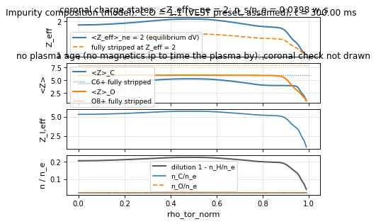
impurity_profile_composition · shot 48224 Staleimpurity_profile_charge_state_fraction
profile
source
impurity / profile / charge_state_fraction · domain core_profiles · view model Panels
Charge-state fractions f_q(rho) of each impurity element from the slice's T_e and n_e.
Thumbnail drawn from sample shot 48224, stale: renderer or style changed.
vaft.omas.plot_impurity_profile_charge_state_fraction(ods) # from data
vaft.plot.impurity_profile_charge_state_fraction(model) # from a PanelsShow source vaft/plot/renderers/panels.py, lines 713–739
@_panel_renderer(
domain="core_profiles",
subject="impurity",
view="profile",
quantity="charge_state_fraction",
description="Charge-state fractions f_q(rho) of each impurity element from the slice's T_e and n_e.",
# equilibrium: the volume of the n_e-weighted mean; magnetics,
# spectrometer_uv, summary: the plasma onset the age is measured from.
ids=("core_profiles", "equilibrium", "magnetics", "spectrometer_uv", "summary"),
required_paths=(
"core_profiles.profiles_1d.{i}.electrons.temperature",
"core_profiles.profiles_1d.{i}.grid.rho_tor_norm",
# n_e in either spelling, which the recipe's `available` predicate checks.
),
optional_paths=(
"core_profiles.profiles_1d.{i}.electrons.density_thermal",
"core_profiles.profiles_1d.{i}.electrons.density",
"core_profiles.profiles_1d.{i}.zeff",
"equilibrium.time_slice.{i}.profiles_1d.volume",
"magnetics.ip.0.data",
),
)
def impurity_profile_charge_state_fraction(
model: Panels, *, ax: Any = None, show: bool = False, **style: Any
) -> tuple[Figure, np.ndarray]:
"""Charge-state fractions f_q(rho) of each impurity element."""
return render_panels(model, ax=ax, show=show, **style)| IDS | core_profiles, equilibrium, magnetics, spectrometer_uv, summary |
|---|---|
| Required paths | core_profiles.profiles_1d.{i}.electrons.temperaturecore_profiles.profiles_1d.{i}.grid.rho_tor_norm |
| Optional paths | core_profiles.profiles_1d.{i}.electrons.density_thermalcore_profiles.profiles_1d.{i}.electrons.densitycore_profiles.profiles_1d.{i}.zeffequilibrium.time_slice.{i}.profiles_1d.volumemagnetics.ip.0.data |
| Backends | matplotlib, plotly |
| Renderer | vaft.plot.renderers.panels.impurity_profile_charge_state_fraction |
impurity_profile_composition
profile
source
impurity / profile / composition · domain core_profiles · view model Panels
Radial Z_eff, mean charges, reduced impurity charge and dilution from the slice's T_e and n_e through atomic-data charge states, for a stated elemental composition.
Thumbnail drawn from sample shot 48224, stale: renderer or style changed.
vaft.omas.plot_impurity_profile_composition(ods) # from data
vaft.plot.impurity_profile_composition(model) # from a PanelsShow source vaft/plot/renderers/panels.py, lines 681–710
@_panel_renderer(
domain="core_profiles",
subject="impurity",
view="profile",
quantity="composition",
description=(
"Radial Z_eff, mean charges, reduced impurity charge and dilution from the slice's "
"T_e and n_e through atomic-data charge states, for a stated elemental composition."
),
# equilibrium: the volume of the n_e-weighted mean; magnetics,
# spectrometer_uv, summary: the plasma onset the age is measured from.
ids=("core_profiles", "equilibrium", "magnetics", "spectrometer_uv", "summary"),
required_paths=(
"core_profiles.profiles_1d.{i}.electrons.temperature",
"core_profiles.profiles_1d.{i}.grid.rho_tor_norm",
# n_e in either spelling, which the recipe's `available` predicate checks.
),
optional_paths=(
"core_profiles.profiles_1d.{i}.electrons.density_thermal",
"core_profiles.profiles_1d.{i}.electrons.density",
"core_profiles.profiles_1d.{i}.zeff",
"equilibrium.time_slice.{i}.profiles_1d.volume",
"magnetics.ip.0.data",
),
)
def impurity_profile_composition(
model: Panels, *, ax: Any = None, show: bool = False, **style: Any
) -> tuple[Figure, np.ndarray]:
"""Radial Z_eff, <Z>, Z_I,eff and dilution from T_e, n_e through ADF11 charge states."""
return render_panels(model, ax=ax, show=show, **style)| IDS | core_profiles, equilibrium, magnetics, spectrometer_uv, summary |
|---|---|
| Required paths | core_profiles.profiles_1d.{i}.electrons.temperaturecore_profiles.profiles_1d.{i}.grid.rho_tor_norm |
| Optional paths | core_profiles.profiles_1d.{i}.electrons.density_thermalcore_profiles.profiles_1d.{i}.electrons.densitycore_profiles.profiles_1d.{i}.zeffequilibrium.time_slice.{i}.profiles_1d.volumemagnetics.ip.0.data |
| Backends | matplotlib, plotly |
| Renderer | vaft.plot.renderers.panels.impurity_profile_composition |
Code subjects
chease
chease_overview_profile_validitychease_overview_refinement_summarychease_overview_profile_validity
overview
source
chease / overview / profile_validity · domain chease · view model Panels
q0/q95, q-monotonicity and pressure positivity of the refined equilibrium: a converged CHEASE solution that is not physically sound flagged at a glance.
No thumbnail: no packaged sample carries the data this plot needs.
vaft.omas.plot_chease_overview_profile_validity(ods) # from data
vaft.plot.chease_overview_profile_validity(model) # from a PanelsShow source vaft/plot/renderers/panels.py, lines 547–565
@_panel_renderer(
domain="chease",
subject="chease",
view="overview",
quantity="profile_validity",
description=(
"q0/q95, q-monotonicity and pressure positivity of the refined "
"equilibrium: a converged CHEASE solution that is not physically "
"sound flagged at a glance."
),
ids=("equilibrium",),
# Same reasoning as the refinement summary.
required_paths=("equilibrium.code.library.0.name",),
)
def chease_overview_profile_validity(
model: Panels, *, ax: Any = None, show: bool = False, **style: Any
) -> tuple[Figure, np.ndarray]:
"""Physical validity of the refined equilibrium's profiles."""
return render_panels(model, ax=ax, show=show, **style)| IDS | equilibrium |
|---|---|
| Required paths | equilibrium.code.library.0.name |
| Backends | matplotlib, plotly |
| Renderer | vaft.plot.renderers.panels.chease_overview_profile_validity |
chease_overview_refinement_summary
overview
source
chease / overview / refinement_summary · domain chease · view model Panels
How far CHEASE moved each profile and the boundary from the EFIT equilibrium it refined, slice by slice: profile and boundary RMS change, flux-normalization shift, and plasma-current self-consistency.
No thumbnail: no packaged sample carries the data this plot needs.
vaft.omas.plot_chease_overview_refinement_summary(ods) # from data
vaft.plot.chease_overview_refinement_summary(model) # from a PanelsShow source vaft/plot/renderers/panels.py, lines 522–544
@_panel_renderer(
domain="chease",
subject="chease",
view="overview",
quantity="refinement_summary",
description=(
"How far CHEASE moved each profile and the boundary from the EFIT "
"equilibrium it refined, slice by slice: profile and boundary RMS "
"change, flux-normalization shift, and plasma-current self-consistency."
),
ids=("equilibrium",),
# `equilibrium.code.name` is not exclusive to CHEASE -- vaft.data.vfit
# also sets it (to "VFIT") -- and the registry's availability check only
# tests path *presence*, not value, so a shared path would offer this
# plot for any equilibrium reconstruction that happens to set code.name.
# `code.library.0.name` is written only by `generate_chease_ods.py`.
required_paths=("equilibrium.code.library.0.name",),
)
def chease_overview_refinement_summary(
model: Panels, *, ax: Any = None, show: bool = False, **style: Any
) -> tuple[Figure, np.ndarray]:
"""CHEASE refinement-vs-input comparison, slice by slice."""
return render_panels(model, ax=ax, show=show, **style)| IDS | equilibrium |
|---|---|
| Required paths | equilibrium.code.library.0.name |
| Backends | matplotlib, plotly |
| Renderer | vaft.plot.renderers.panels.chease_overview_refinement_summary |
Composite subjects
current
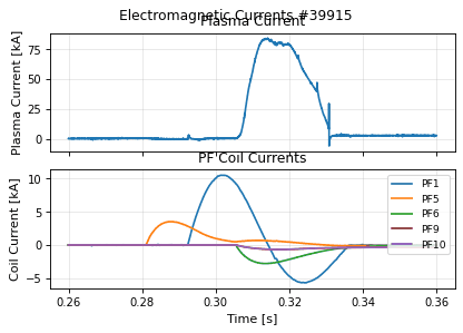
current_overview · shot 39915 Stale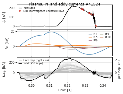
current_overview_reconstruction · shot 41524 Stalecurrent_overview
overview
source
current / overview · domain electromagnetics · view model Panels
Plasma, PF coil and eddy current panels on a shared time axis.
Thumbnail drawn from sample shot 39915, stale: renderer or style changed.
vaft.omas.plot_current_overview(ods) # from data
vaft.plot.current_overview(model) # from a PanelsShow source vaft/plot/renderers/panels.py, lines 798–811
@_panel_renderer(
domain="electromagnetics",
subject="current",
view="overview",
quantity="",
description="Plasma, PF coil and eddy current panels on a shared time axis.",
ids=("magnetics", "pf_active", "pf_passive"),
required_paths=("magnetics.ip.0.data",),
)
def current_overview(
model: Panels, *, ax: Any = None, show: bool = False, **style: Any
) -> tuple[Figure, np.ndarray]:
"""Plasma, PF coil and eddy current panels on a shared time axis."""
return render_panels(model, ax=ax, show=show, **style)| IDS | magnetics, pf_active, pf_passive |
|---|---|
| Required paths | magnetics.ip.0.data |
| Backends | matplotlib, plotly |
| Renderer | vaft.plot.renderers.panels.current_overview |
current_overview_reconstruction
overview
source
current / overview / reconstruction · domain electromagnetics · view model Panels
Measured I_p with the reconstructed I_p of every equilibrium slice by convergence, PF coil currents and eddy currents, in kA.
Interpretation
The three currents that set the poloidal field of a VEST discharge, on one time axis. The top panel is the Rogowski plasma current with, as markers at each slice’s time, the plasma current the equilibrium reconstruction fitted: filled where the solver’s evidence says the slice converged, a cross where it says it did not, hollow where no evidence was stored. A marker on the trace says the reconstruction matched the measured current; one off it, or a cross, says that slice should not be read further. The middle panel is each PF coil’s current as stored, per turn. The bottom panel is the current induced in the vessel and passive structure: their total strong against the left axis, and every loop faint against a right-hand axis of its own, since one loop carries about a hundredth of the total and would otherwise vanish onto zero. In the Matplotlib figure the two axes put their zero at the same height whenever both ranges straddle it, so a loop and the total read above or below it the same way; their scales differ. Without an equilibrium the top panel is the measured current alone.
Limitations
The eddy currents are a circuit-model solution (pf_passive from
vaft.omas.compute_eddy_currents), not a measurement. Convergence is
the solver’s own evidence as vaft.validation.equilibrium.
verify_convergence reads it; a converged slice can still fit the
magnetics poorly, which equilibrium_overview_fit_quality shows. PF
coils that carry no current at all in the shot are not drawn;
pf_coil_time_current draws every coil. A loop sample that is not
finite is left out of the total at that time, and the total is missing
only where no loop is finite. The 6.5 in column keeps the format’s type
size, so a poster figure is tall and narrow; pass figsize= there.
Convention · See Also
Convention
Currents are in kA. The PF panel is the stored coil current, per turn
(pf_coil_time_current_turns multiplies it by the turns). The PF and
eddy panels keep the IMAS sign; only the plasma
current is re-signed for display, and the figure title says so when it is.
See Also
current_overview : the same three currents in A, one trace per coil and the eddy total. equilibrium_overview_convergence : the convergence evidence behind the markers. passive_structure_time_current : the eddy current alone, or selected loops.
Thumbnail drawn from sample shot 41524, stale: renderer or style changed.
vaft.omas.plot_current_overview_reconstruction(ods) # from data
vaft.plot.current_overview_reconstruction(model) # from a Panels| IDS | magnetics, pf_active, pf_passive, equilibrium |
|---|---|
| Required paths | magnetics.ip.0.datapf_active.coil.{i}.current.datapf_passive.timepf_passive.loop.{i}.current |
| Optional paths | equilibrium.time_slice.{i}.global_quantities.ip |
| Backends | matplotlib, plotly |
| Renderer | vaft.plot.renderers.panels.current_overview_reconstruction |
diagnostics
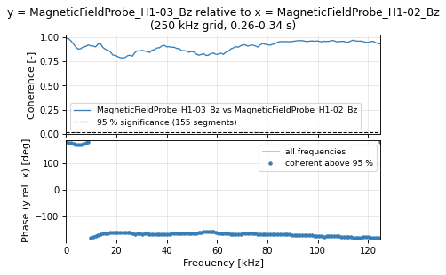
diagnostics_spectrum_coherence · shot 39915 Stale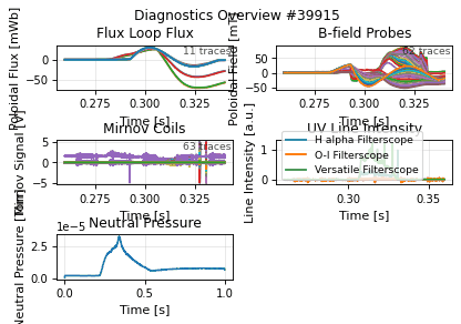
diagnostics_overview · shot 39915 Stalediagnostics_spectrum_coherence
spectrum
source
diagnostics / spectrum / coherence · domain magnetics · view model Panels
Coherence (with its 95 % significance line) and relative phase of two fluctuation channels – Mirnov, soft X-ray or interferometer – compared on one time grid over their overlap (issue #1005).
Thumbnail drawn from sample shot 39915, stale: renderer or style changed.
vaft.omas.plot_diagnostics_spectrum_coherence(ods) # from data
vaft.plot.diagnostics_spectrum_coherence(model) # from a PanelsShow source vaft/plot/renderers/spectra.py, lines 195–227
@renderer(
domain="magnetics",
subject="diagnostics",
view="spectrum",
quantity="coherence",
model=Panels,
description=(
"Coherence (with its 95 % significance line) and relative phase of two "
"fluctuation channels -- Mirnov, soft X-ray or interferometer -- compared "
"on one time grid over their overlap (issue #1005)."
),
ids=("magnetics", "soft_x_rays", "interferometer"),
optional_paths=(
"magnetics.b_field_pol_probe.{i}.voltage.data",
"magnetics.b_field_pol_probe.{i}.voltage.time",
"magnetics.time",
"soft_x_rays.channel.{i}.brightness.data",
"soft_x_rays.channel.{i}.brightness.time",
"soft_x_rays.channel.{i}.power.data",
"soft_x_rays.channel.{i}.power.time",
"soft_x_rays.time",
"interferometer.channel.{i}.n_e_line.data",
"interferometer.channel.{i}.n_e_line.time",
"interferometer.time",
),
)
def diagnostics_spectrum_coherence(
model: Panels, *, ax: Any = None, show: bool = False, **style: Any
) -> tuple[Figure, Any]:
"""Coherence and relative phase of two fluctuation channels."""
from .panels import render_panels
return render_panels(model, ax=ax, show=show, **style)| IDS | magnetics, soft_x_rays, interferometer |
|---|---|
| Required paths | — |
| Optional paths | magnetics.b_field_pol_probe.{i}.voltage.datamagnetics.b_field_pol_probe.{i}.voltage.timemagnetics.timesoft_x_rays.channel.{i}.brightness.datasoft_x_rays.channel.{i}.brightness.timesoft_x_rays.channel.{i}.power.datasoft_x_rays.channel.{i}.power.timesoft_x_rays.timeinterferometer.channel.{i}.n_e_line.datainterferometer.channel.{i}.n_e_line.timeinterferometer.time |
| Backends | matplotlib, plotly |
| Renderer | vaft.plot.renderers.spectra.diagnostics_spectrum_coherence |
diagnostics_overview
overview
source
diagnostics / overview · domain magnetics · view model Panels
Time histories of every diagnostic subject, one panel each; a diagnostic absent from the input is left out and the grid shrinks (issue #476), and members= picks the panels by name (issue #482). Channels the source flagged invalid are excluded by default.
Thumbnail drawn from sample shot 39915, stale: renderer or style changed.
vaft.omas.plot_diagnostics_overview(ods) # from data
vaft.plot.diagnostics_overview(model) # from a PanelsShow source vaft/plot/renderers/panels.py, lines 944–963
@_panel_renderer(
domain="magnetics",
subject="diagnostics",
view="overview",
quantity="",
description=(
"Time histories of every diagnostic subject, one panel each; a "
"diagnostic absent from the input is left out and the grid shrinks "
"(issue #476), and members= picks the panels by name (issue #482). "
"Channels the source flagged invalid are excluded by default."
),
ids=("magnetics", "interferometer", "thomson_scattering", "charge_exchange",
"spectrometer_uv", "barometry", "soft_x_rays"),
required_paths=(),
)
def diagnostics_overview(
model: Panels, *, ax: Any = None, show: bool = False, **style: Any
) -> tuple[Figure, np.ndarray]:
"""Fixed-shape time overview across the diagnostic subjects."""
return render_panels(model, ax=ax, show=show, **style)| IDS | magnetics, interferometer, thomson_scattering, charge_exchange, spectrometer_uv, barometry, soft_x_rays |
|---|---|
| Required paths | — |
| Backends | matplotlib, plotly |
| Renderer | vaft.plot.renderers.panels.diagnostics_overview |
kinetic
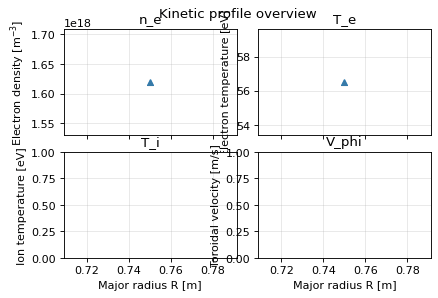
kinetic_overview_profiles · shot 40600 Stale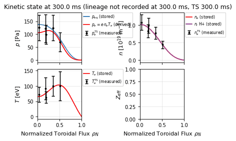
kinetic_overview_state · shot 48224 Stalekinetic_overview_profiles
overview
source
kinetic / overview / profiles · domain diagnostics · view model Panels
Local n_e, T_e, T_i and V_phi from compatible diagnostics and core-profile fits.
Thumbnail drawn from sample shot 40600, stale: renderer or style changed.
vaft.omas.plot_kinetic_overview_profiles(ods) # from data
vaft.plot.kinetic_overview_profiles(model) # from a PanelsShow source vaft/plot/renderers/panels.py, lines 966–977
@_panel_renderer(
domain="diagnostics", subject="kinetic", view="overview", quantity="profiles",
description="Local n_e, T_e, T_i and V_phi from compatible diagnostics and core-profile fits.",
ids=("thomson_scattering", "charge_exchange", "langmuir_probes", "core_profiles", "equilibrium"),
required_paths=(),
)
def kinetic_overview_profiles(
model: Panels, *, ax: Any = None, show: bool = False, **style: Any
) -> tuple[Figure, np.ndarray]:
"""Four cross-diagnostic kinetic profile panels."""
style.setdefault("figsize", (14.0, 7.0))
return render_panels(model, ax=ax, show=show, **style)| IDS | thomson_scattering, charge_exchange, langmuir_probes, core_profiles, equilibrium |
|---|---|
| Required paths | — |
| Backends | matplotlib, plotly |
| Renderer | vaft.plot.renderers.panels.kinetic_overview_profiles |
kinetic_overview_state
overview
source
kinetic / overview / state · domain core_profiles · view model Panels
One matched kinetic state in four panels – pressure, density, temperature and Z_eff against rho_tor_norm – from stored core_profiles, the equilibrium of the same time and the Thomson channels mapped through it, each trace labelled by its recorded evidence role.
Interpretation
The four views of a single selected kinetic state, on one radial coordinate. Pressure compares the equilibrium pressure with the electron and ion pressures stored in core_profiles and their sum; density shows the electron, main-ion and charged impurity-ion densities; temperature the electron and ion temperatures; the last panel the effective charge with its stored resistive value or the recorded composition target as a reference. Thomson channels are mapped from their own (R, Z) through the selected equilibrium and drawn with their 1 sigma errors; where no channel lies, every profile is extrapolated. Each legend entry names the role its quantity’s provenance record states – measurement, fit, assumed, inferred – and the plot derives two more from the records: Thomson points are the fit input of fitted profiles, and the Thomson pressure is independent validation of a magnetics-only equilibrium but fit input of an electron-kinetic one. p_e + p_i is labelled a closure identity when T_i was inferred by partitioning the equilibrium pressure, because it then equals p_eq by construction and is no agreement test. A stored impurity pressure is drawn as the part of p_i it is (p_i is the total over every ion), never added to the sum again. What the records say was assumed – T_i = T_e, n_C = n_O, a preset Z_eff target – is listed under the title, and the resistive (Romero) Z_eff a composition was closed on, with its sigma, on an “Inferred” line below it.
The figure can also be read as the inference chain that built the state: Thomson and equilibrium data (1), the n_e and T_e fits (2), T_i (3), the Z_eff reference such as Romero’s resistive estimate (4), the impurity density (5), the main-ion density (6), the Z_eff profile (7) and the pressure closure (8). The stage of a trace is fixed by its quantity, not by the data, so a state built in another order is drawn as stored.
Limitations
Nothing is computed beyond presentation: ion densities, T_i and Z_eff are what the stage stored, and by design no uncertainty band is drawn on p_eq, p_i, T_i, the ion densities or Z_eff – the contract carries none for them. The Thomson pressure error assumes independent n_e and T_e errors. A quantity without a provenance record is labelled “stored” (a Thomson channel “measured”), not guessed; a record in no known grammar is refused. Non-finite T_i, p_i and Z_eff points stay empty. On a canvas narrower than 6 inches the legends move inside the panels and may cover data. The stages layout’s legends name symbols only; the roles are the single figure’s to state.
See Also
See Also
kinetic_overview_profiles : local Thomson/CX points and the core-profile fits. core_profiles_profile_zeff : the stored Z_eff alone, labelled by its origin.
Thumbnail drawn from sample shot 48224, stale: renderer or style changed.
vaft.omas.plot_kinetic_overview_state(ods) # from data
vaft.plot.kinetic_overview_state(model) # from a Panels| IDS | core_profiles, equilibrium, thomson_scattering |
|---|---|
| Required paths | core_profiles.profiles_1d.{i}.grid.rho_tor_normcore_profiles.profiles_1d.{i}.electrons.densitycore_profiles.profiles_1d.{i}.electrons.temperature |
| Optional paths | equilibrium.time_slice.{i}.profiles_1d.pressurecore_profiles.profiles_1d.{i}.t_i_averagecore_profiles.profiles_1d.{i}.pressure_ion_totalcore_profiles.profiles_1d.{i}.ion.{j}.densitycore_profiles.profiles_1d.{i}.ion.{j}.pressurecore_profiles.profiles_1d.{i}.ion.{j}.temperature_fit.parameterscore_profiles.profiles_1d.{i}.zeffcore_profiles.profiles_1d.{i}.zeff_fit.parameterscore_profiles.global_quantities.z_eff_resistivethomson_scattering.channel.{i}.n_e.datathomson_scattering.channel.{i}.t_e.data |
| Backends | matplotlib, plotly |
| Renderer | vaft.plot.renderers.panels.kinetic_overview_state |
summary
summary_time_energy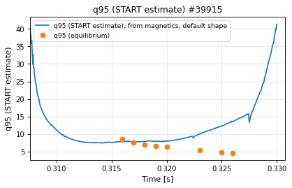
summary_time_estimated_q95 · shot 39915 Stale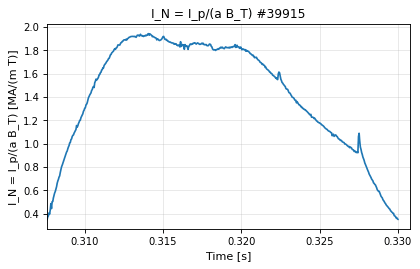
summary_time_normalized_current · shot 39915 Stalesummary_time_power_balance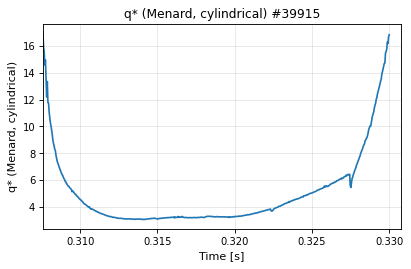
summary_time_q_star_cylindrical · shot 39915 Stale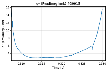
summary_time_q_star_kink · shot 39915 Stalesummary_time_resistive_zeff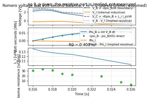
summary_time_romero_balance · shot 39915 Stale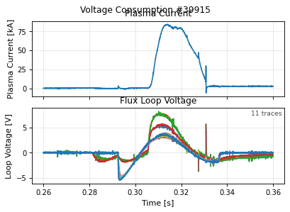
summary_time_voltage_consumption · shot 39915 Stalesummary_time_energy
time
source
summary / time / energy · domain summary · view model Panels
Stored-energy comparison panels across available estimates.
No thumbnail: no packaged sample carries the data this plot needs.
vaft.omas.plot_summary_time_energy(ods) # from data
vaft.plot.summary_time_energy(model) # from a PanelsShow source vaft/plot/renderers/panels.py, lines 568–581
@_panel_renderer(
domain="summary",
subject="summary",
view="time",
quantity="energy",
description="Stored-energy comparison panels across available estimates.",
ids=("equilibrium", "core_profiles", "magnetics"),
required_paths=("equilibrium.time",),
)
def summary_time_energy(
model: Panels, *, ax: Any = None, show: bool = False, **style: Any
) -> tuple[Figure, np.ndarray]:
"""Stored-energy comparison panels across available estimates."""
return render_panels(model, ax=ax, show=show, **style)| IDS | equilibrium, core_profiles, magnetics |
|---|---|
| Required paths | equilibrium.time |
| Backends | matplotlib, plotly |
| Renderer | vaft.plot.renderers.panels.summary_time_energy |
summary_time_estimated_q95
time
source
summary / time / estimated_q95 · domain summary · view model LineSeries
q95 estimated from global shape, I_p and B_T (START scaling by default, from vest.yaml), the equilibrium q95 overlaid; works without an equilibrium (issue #1583).
Thumbnail drawn from sample shot 39915, stale: renderer or style changed.
vaft.omas.plot_summary_time_estimated_q95(ods) # from data
vaft.plot.summary_time_estimated_q95(model) # from a LineSeriesShow source vaft/plot/renderers/edge_q.py, lines 56–65
@_edge_q_renderer(
"estimated_q95",
"q95 estimated from global shape, I_p and B_T (START scaling by default, from vest.yaml), "
"the equilibrium q95 overlaid; works without an equilibrium (issue #1583).",
)
def summary_time_estimated_q95(
model: LineSeries, *, ax: Axes | None = None, show: bool = False, **style: Any
) -> tuple[Figure, Axes]:
"""Estimated q95 against time, labelled with its scaling, equilibrium q95 overlaid."""
return render_line_series(model, ax=ax, show=show, **style)| IDS | equilibrium, magnetics, tf |
|---|---|
| Required paths | — |
| Optional paths | equilibrium.timeequilibrium.time_slice.{i}.boundary.outline.requilibrium.time_slice.{i}.global_quantities.ipequilibrium.time_slice.{i}.global_quantities.q_95equilibrium.vacuum_toroidal_field.b0magnetics.ip.0.datatf.b_field_tor_vacuum_r.data |
| Backends | matplotlib, plotly |
| Renderer | vaft.plot.renderers.edge_q.summary_time_estimated_q95 |
summary_time_normalized_current
time
source
summary / time / normalized_current · domain summary · view model LineSeries
Normalised current I_N = I_p[MA]/(a B_T) against time, from the same shape as the edge-q estimates (issue #1583).
Thumbnail drawn from sample shot 39915, stale: renderer or style changed.
vaft.omas.plot_summary_time_normalized_current(ods) # from data
vaft.plot.summary_time_normalized_current(model) # from a LineSeriesShow source vaft/plot/renderers/edge_q.py, lines 92–101
@_edge_q_renderer(
"normalized_current",
"Normalised current I_N = I_p[MA]/(a B_T) against time, from the same shape as the "
"edge-q estimates (issue #1583).",
)
def summary_time_normalized_current(
model: LineSeries, *, ax: Axes | None = None, show: bool = False, **style: Any
) -> tuple[Figure, Axes]:
"""Normalised current I_N against time."""
return render_line_series(model, ax=ax, show=show, **style)| IDS | equilibrium, magnetics, tf |
|---|---|
| Required paths | — |
| Optional paths | equilibrium.timeequilibrium.time_slice.{i}.boundary.outline.requilibrium.time_slice.{i}.global_quantities.ipequilibrium.time_slice.{i}.global_quantities.q_95equilibrium.vacuum_toroidal_field.b0magnetics.ip.0.datatf.b_field_tor_vacuum_r.data |
| Backends | matplotlib, plotly |
| Renderer | vaft.plot.renderers.edge_q.summary_time_normalized_current |
summary_time_power_balance
time
source
summary / time / power_balance · domain summary · view model Panels
Ohmic input, radiated and conducted power balance panels.
No thumbnail: no packaged sample carries the data this plot needs.
vaft.omas.plot_summary_time_power_balance(ods) # from data
vaft.plot.summary_time_power_balance(model) # from a PanelsShow source vaft/plot/renderers/panels.py, lines 642–658
@_panel_renderer(
domain="summary",
subject="summary",
view="time",
quantity="power_balance",
description="Ohmic input, radiated and conducted power balance panels.",
ids=("equilibrium", "core_profiles", "summary"),
required_paths=(
"equilibrium.time_slice.{i}.global_quantities.ip",
"equilibrium.time_slice.{i}.global_quantities.volume",
),
)
def summary_time_power_balance(
model: Panels, *, ax: Any = None, show: bool = False, **style: Any
) -> tuple[Figure, np.ndarray]:
"""Ohmic input, radiated and conducted power balance panels."""
return render_panels(model, ax=ax, show=show, **style)| IDS | equilibrium, core_profiles, summary |
|---|---|
| Required paths | equilibrium.time_slice.{i}.global_quantities.ipequilibrium.time_slice.{i}.global_quantities.volume |
| Backends | matplotlib, plotly |
| Renderer | vaft.plot.renderers.panels.summary_time_power_balance |
summary_time_q_star_cylindrical
time
source
summary / time / q_star_cylindrical · domain summary · view model LineSeries
Menard's cylindrical safety factor q* = pi a^2 B_T (1 + kappa^2)/(mu0 R I_p) against time; a shape-weighted proxy, not q95 or q_a (issue #1583).
Thumbnail drawn from sample shot 39915, stale: renderer or style changed.
vaft.omas.plot_summary_time_q_star_cylindrical(ods) # from data
vaft.plot.summary_time_q_star_cylindrical(model) # from a LineSeriesShow source vaft/plot/renderers/edge_q.py, lines 68–77
@_edge_q_renderer(
"q_star_cylindrical",
"Menard's cylindrical safety factor q* = pi a^2 B_T (1 + kappa^2)/(mu0 R I_p) against time; "
"a shape-weighted proxy, not q95 or q_a (issue #1583).",
)
def summary_time_q_star_cylindrical(
model: LineSeries, *, ax: Axes | None = None, show: bool = False, **style: Any
) -> tuple[Figure, Axes]:
"""Menard's cylindrical q* against time."""
return render_line_series(model, ax=ax, show=show, **style)| IDS | equilibrium, magnetics, tf |
|---|---|
| Required paths | — |
| Optional paths | equilibrium.timeequilibrium.time_slice.{i}.boundary.outline.requilibrium.time_slice.{i}.global_quantities.ipequilibrium.time_slice.{i}.global_quantities.q_95equilibrium.vacuum_toroidal_field.b0magnetics.ip.0.datatf.b_field_tor_vacuum_r.data |
| Backends | matplotlib, plotly |
| Renderer | vaft.plot.renderers.edge_q.summary_time_q_star_cylindrical |
summary_time_q_star_kink
time
source
summary / time / q_star_kink · domain summary · view model LineSeries
Freidberg's kink safety factor q* = 2 pi a^2 kappa B_T/(mu0 R I_p) against time; not q95 or q_a (issue #1583).
Thumbnail drawn from sample shot 39915, stale: renderer or style changed.
vaft.omas.plot_summary_time_q_star_kink(ods) # from data
vaft.plot.summary_time_q_star_kink(model) # from a LineSeriesShow source vaft/plot/renderers/edge_q.py, lines 80–89
@_edge_q_renderer(
"q_star_kink",
"Freidberg's kink safety factor q* = 2 pi a^2 kappa B_T/(mu0 R I_p) against time; "
"not q95 or q_a (issue #1583).",
)
def summary_time_q_star_kink(
model: LineSeries, *, ax: Axes | None = None, show: bool = False, **style: Any
) -> tuple[Figure, Axes]:
"""Freidberg's kink q* against time."""
return render_line_series(model, ax=ax, show=show, **style)| IDS | equilibrium, magnetics, tf |
|---|---|
| Required paths | — |
| Optional paths | equilibrium.timeequilibrium.time_slice.{i}.boundary.outline.requilibrium.time_slice.{i}.global_quantities.ipequilibrium.time_slice.{i}.global_quantities.q_95equilibrium.vacuum_toroidal_field.b0magnetics.ip.0.datatf.b_field_tor_vacuum_r.data |
| Backends | matplotlib, plotly |
| Renderer | vaft.plot.renderers.edge_q.summary_time_q_star_kink |
summary_time_resistive_zeff
time
source
summary / time / resistive_zeff · domain summary · view model Panels
Resistive Z_eff history: Romero voltages, observed vs model R_p, window estimate.
No thumbnail: shot 48224: ValueError: fewer than three consecutive current-carrying equilibrium slices.
vaft.omas.plot_summary_time_resistive_zeff(ods) # from data
vaft.plot.summary_time_resistive_zeff(model) # from a PanelsShow source vaft/plot/renderers/panels.py, lines 661–678
@_panel_renderer(
domain="summary",
subject="summary",
view="time",
quantity="resistive_zeff",
description="Resistive Z_eff history: Romero voltages, observed vs model R_p, window estimate.",
ids=("equilibrium", "core_profiles"),
required_paths=(
"equilibrium.time_slice.{i}.global_quantities.ip",
"equilibrium.time_slice.{i}.profiles_1d.f_df_dpsi",
"core_profiles.profiles_1d.{i}.electrons.temperature",
),
)
def summary_time_resistive_zeff(
model: Panels, *, ax: Any = None, show: bool = False, **style: Any
) -> tuple[Figure, np.ndarray]:
"""Resistive Z_eff history: Romero voltages, observed vs model R_p, window estimate."""
return render_panels(model, ax=ax, show=show, **style)| IDS | equilibrium, core_profiles |
|---|---|
| Required paths | equilibrium.time_slice.{i}.global_quantities.ipequilibrium.time_slice.{i}.profiles_1d.f_df_dpsicore_profiles.profiles_1d.{i}.electrons.temperature |
| Backends | matplotlib, plotly |
| Renderer | vaft.plot.renderers.panels.summary_time_resistive_zeff |
summary_time_romero_balance
time
source
summary / time / romero_balance · domain summary · view model Panels
Romero's voltage and volt-second balance: V_B, V_I, V_C (and V_R with a given R_p), Phi_B against the direct flux change, L_i and the closing resistance.
Thumbnail drawn from sample shot 39915, stale: renderer or style changed.
vaft.omas.plot_summary_time_romero_balance(ods) # from data
vaft.plot.summary_time_romero_balance(model) # from a PanelsShow source vaft/plot/renderers/panels.py, lines 742–763
@_panel_renderer(
domain="summary",
subject="summary",
view="time",
quantity="romero_balance",
description=(
"Romero's voltage and volt-second balance: V_B, V_I, V_C (and V_R with a given R_p), "
"Phi_B against the direct flux change, L_i and the closing resistance."
),
ids=("equilibrium", "tf", "wall"),
required_paths=(
"equilibrium.time_slice.{i}.global_quantities.ip",
"equilibrium.time_slice.{i}.global_quantities.psi_boundary",
"equilibrium.time_slice.{i}.global_quantities.psi_axis",
"equilibrium.time_slice.{i}.profiles_2d.0.psi",
),
)
def summary_time_romero_balance(
model: Panels, *, ax: Any = None, show: bool = False, **style: Any
) -> tuple[Figure, np.ndarray]:
"""Romero's voltage and volt-second balance."""
return render_panels(model, ax=ax, show=show, **style)| IDS | equilibrium, tf, wall |
|---|---|
| Required paths | equilibrium.time_slice.{i}.global_quantities.ipequilibrium.time_slice.{i}.global_quantities.psi_boundaryequilibrium.time_slice.{i}.global_quantities.psi_axisequilibrium.time_slice.{i}.profiles_2d.0.psi |
| Backends | matplotlib, plotly |
| Renderer | vaft.plot.renderers.panels.summary_time_romero_balance |
summary_time_voltage_consumption
time
source
summary / time / voltage_consumption · domain summary · view model Panels
Loop-voltage and flux-consumption panels.
Thumbnail drawn from sample shot 39915, stale: renderer or style changed.
vaft.omas.plot_summary_time_voltage_consumption(ods) # from data
vaft.plot.summary_time_voltage_consumption(model) # from a PanelsShow source vaft/plot/renderers/panels.py, lines 766–779
@_panel_renderer(
domain="summary",
subject="summary",
view="time",
quantity="voltage_consumption",
description="Loop-voltage and flux-consumption panels.",
ids=("magnetics", "pf_active"),
required_paths=("magnetics.time",),
)
def summary_time_voltage_consumption(
model: Panels, *, ax: Any = None, show: bool = False, **style: Any
) -> tuple[Figure, np.ndarray]:
"""Loop-voltage and flux-consumption panels."""
return render_panels(model, ax=ax, show=show, **style)| IDS | magnetics, pf_active |
|---|---|
| Required paths | magnetics.time |
| Backends | matplotlib, plotly |
| Renderer | vaft.plot.renderers.panels.summary_time_voltage_consumption |
Other plotting functions
Plotting functions vaft.plot offers outside the registry: ad-hoc and analytic figures that take a
result rather than an ODS (support), and the cross-shot statistics kept as they are until they get a
canonical home (legacy). They have no subject / view identity and no vaft.omas adapter.
plot_cross_diagnostic_coherence_spectrogram
Support
source
vaft.plot.plot_cross_diagnostic_coherence_spectrogram(result, *, ax=None, show=False)Show source vaft/plot/fluctuation.py, lines 69–77
def plot_cross_diagnostic_coherence_spectrogram(
result: Any, *, ax: Any = None, show: bool = False,
) -> tuple[Any, Any]:
"""Time-resolved magnitude-squared coherence of two selected signals."""
return _fluctuation_map(
result, result.coherence, title="Cross-diagnostic coherence",
colorbar="Magnitude-squared coherence", cmap="viridis",
vmin=0, vmax=1, ax=ax, show=show,
)Time-resolved magnitude-squared coherence of two selected signals.
Defined in vaft.plot.fluctuation
plot_cross_spectrum
Support
source
vaft.plot.plot_cross_spectrum(result, *, x_label='x', y_label='y', title=None, max_frequency=None, ax=None, show=False, **style)Show source vaft/plot/fluctuation.py, lines 235–256
def plot_cross_spectrum(
result: Any,
*,
x_label: str = "x",
y_label: str = "y",
title: str | None = None,
max_frequency: float | None = None,
ax: Any = None,
show: bool = False,
**style: Any,
) -> tuple[Any, Any]:
"""Draw a :class:`~vaft.process.fluctuation.CrossSpectrum`; returns ``(Figure, axes)``.
Two panels: magnitude-squared coherence with the 95 % significance line, and
the phase of ``y`` relative to ``x``. ``ax`` may supply the two axes.
"""
from .renderers.panels import render_panels
model = cross_spectrum_model(
result, x_label=x_label, y_label=y_label, title=title, max_frequency=max_frequency
)
return render_panels(model, ax=ax, show=show, **style)Draw a :class:~vaft.process.fluctuation.CrossSpectrum; returns (Figure, axes).
Defined in vaft.plot.fluctuation
plot_fluctuation_frequency_coverage
Support
source
vaft.plot.plot_fluctuation_frequency_coverage(diagnostics=None, phenomena=None, *, f_min=1.0, f_max=2000000.0, caption='Phenomenon bands: typical order of magnitude, not an identification rule. Diagnostic bars end at the Nyquist frequency; the usable band is lower (sensor response, filtering, exposure, SNR, line integration).', ax=None, show=False, figsize=None)Show source vaft/plot/fluctuation.py, lines 265–339
def plot_fluctuation_frequency_coverage(
diagnostics: Mapping[str, Any] | None = None,
phenomena: Mapping[str, tuple[float, float] | None] | None = None,
*,
f_min: float = 1.0,
f_max: float = 2e6,
caption: str | None = COVERAGE_CAPTION,
ax: Any = None,
show: bool = False,
figsize: tuple[float, float] | None = None,
) -> tuple[Any, Any]:
"""Diagnostics' Nyquist frequencies against typical phenomenon bands, on log frequency.
``diagnostics`` maps a label to ``(sample_rate, nyquist)`` -- what
:func:`vaft.omas.fluctuation_bandwidths` returns -- or to a Nyquist frequency
alone, in hertz. Each is drawn as a bar from ``f_min`` to its Nyquist
frequency with the value written at the end. ``phenomena`` maps a label to a
``(f_low, f_high)`` band in hertz, or ``None`` for a phenomenon with no single
band (drawn hatched across the whole axis); the default is
:data:`TYPICAL_PHENOMENON_BANDS`. ``caption`` is printed under the axes; pass
``None`` to omit it -- but the bands are order-of-magnitude guidance and the
figure should not be shown without that said somewhere.
"""
from .style import finalize, resolve_axes
diagnostics = dict(diagnostics or {})
phenomena = dict(TYPICAL_PHENOMENON_BANDS if phenomena is None else phenomena)
rows = len(diagnostics) + len(phenomena)
if rows == 0:
raise ValueError("nothing to draw: pass diagnostics= and/or phenomena=")
height = 1.2 + 0.38 * rows + (0.5 if caption else 0.0)
figure, axes = resolve_axes(ax, figsize=figsize or (8.5, height))
labels: list[str] = []
position = rows - 1
phenomenon_colour = resolve_color("emphasis:low")
for label, band in phenomena.items():
if band is None:
axes.barh(position, np.log10(f_max) - np.log10(f_min), left=np.log10(f_min), height=0.6,
color="none", edgecolor=phenomenon_colour, hatch="//", linewidth=0.8)
else:
low, high = float(band[0]), float(band[1])
axes.barh(position, np.log10(high) - np.log10(low), left=np.log10(low), height=0.6,
color=phenomenon_colour, alpha=0.55, edgecolor=phenomenon_colour)
labels.append(label)
position -= 1
if phenomena and diagnostics:
axes.axhline(position + 0.5, color=resolve_color("emphasis:faint"), linewidth=0.8)
for index, (label, value) in enumerate(diagnostics.items()):
nyquist = _nyquist(value)
colour = resolve_color(palette(index))
axes.barh(position, np.log10(nyquist) - np.log10(f_min), left=np.log10(f_min), height=0.6,
color=colour, alpha=0.85)
text = f"f_N = {nyquist / 1e3:.4g} kHz" if nyquist < 1e6 else f"f_N = {nyquist / 1e6:.4g} MHz"
axes.text(np.log10(nyquist), position, f" {text}", va="center", ha="left", fontsize=8)
labels.append(label)
position -= 1
axes.set_yticks(np.arange(rows)[::-1])
axes.set_yticklabels(labels)
decades = np.arange(np.floor(np.log10(f_min)), np.ceil(np.log10(f_max)) + 1)
axes.set_xticks(decades)
axes.set_xticklabels([_decade_label(d) for d in decades])
axes.set_xlim(np.log10(f_min), np.log10(f_max) + 0.9)
axes.set_ylim(-0.7, rows - 0.3)
# The caption rides on the axis label so a tight layout keeps room for it.
xlabel = "Frequency"
if caption:
import textwrap
xlabel += "\n\n" + "\n".join(textwrap.wrap(caption, 70))
axes.set_xlabel(xlabel, fontsize=9 if caption else None)
axes.grid(axis="x", alpha=0.3)
axes.set_title("Fluctuation frequency coverage")
return finalize(figure, axes, show=show, tight_layout=ax is None)Diagnostics’ Nyquist frequencies against typical phenomenon bands, on log frequency.
Defined in vaft.plot.fluctuation
plot_miller_surfaces
Support
source
vaft.plot.plot_miller_surfaces(surfaces, *, ax=None, show=False, theta_points=256, labels=None, title=None, **style)Show source vaft/plot/analytic.py, lines 106–118
def plot_miller_surfaces(
surfaces: Any, *, ax: Any = None, show: bool = False, theta_points: int = 256,
labels: Sequence[str] | None = None, title: str | None = None, **style: Any,
):
"""Draw Miller flux surfaces; returns ``(Figure, Axes)``.
See :func:`miller_surfaces_model` for what is drawn; ``style`` goes to
:func:`vaft.plot.render_geometry_layers`.
"""
from .renderers.geometry import render_geometry_layers
model = miller_surfaces_model(surfaces, theta_points=theta_points, labels=labels, title=title)
return render_geometry_layers(model, ax=ax, show=show, **style)Draw Miller flux surfaces; returns (Figure, Axes).
Defined in vaft.plot.analytic
plot_multi_diagnostic_coherent_fraction
Support
source
vaft.plot.plot_multi_diagnostic_coherent_fraction(result, *, ax=None, show=False)Show source vaft/plot/fluctuation.py, lines 92–101
def plot_multi_diagnostic_coherent_fraction(
result: Any, *, ax: Any = None, show: bool = False,
) -> tuple[Any, Any]:
"""Leading fraction; finite-sample bias means it is not a mode test."""
return _fluctuation_map(
result, result.coherent_fraction,
title="Dominant spectral fraction (compare with a null model)",
colorbar="Leading fraction [dimensionless]", cmap="viridis",
vmin=0, vmax=1, ax=ax, show=show,
)Leading fraction; finite-sample bias means it is not a mode test.
Defined in vaft.plot.fluctuation
plot_multi_diagnostic_coherent_spectrogram
Support
source
vaft.plot.plot_multi_diagnostic_coherent_spectrogram(result, *, ax=None, show=False)Show source vaft/plot/fluctuation.py, lines 80–89
def plot_multi_diagnostic_coherent_spectrogram(
result: Any, *, ax: Any = None, show: bool = False,
) -> tuple[Any, Any]:
"""Leading PSD-normalized spectral eigenvalue, not a physical mode power."""
return _fluctuation_map(
result, result.dominant_power,
title="Dominant coherent spectral component (normalized)",
colorbar="Leading eigenvalue [dimensionless]", cmap="magma",
vmin=0, ax=ax, show=show,
)Leading PSD-normalized spectral eigenvalue, not a physical mode power.
Defined in vaft.plot.fluctuation
plot_multi_diagnostic_participation
Support
source
vaft.plot.plot_multi_diagnostic_participation(result, diagnostic, *, ax=None, show=False)Show source vaft/plot/fluctuation.py, lines 110–120
def plot_multi_diagnostic_participation(
result: Any, diagnostic: str, *, ax: Any = None, show: bool = False,
) -> tuple[Any, Any]:
"""Selected diagnostic's squared dominant-eigenvector loading, not amplitude."""
index = _diagnostic_index(result, diagnostic)
return _fluctuation_map(
result, result.participation[:, :, index],
title=f"{diagnostic}: dimensionless diagnostic participation",
colorbar="Squared loading [dimensionless]", cmap="viridis",
vmin=0, vmax=1, ax=ax, show=show,
)Selected diagnostic’s squared dominant-eigenvector loading, not amplitude.
Defined in vaft.plot.fluctuation
plot_multi_diagnostic_phase
Support
source
vaft.plot.plot_multi_diagnostic_phase(result, diagnostic, *, ax=None, show=False)Show source vaft/plot/fluctuation.py, lines 123–133
def plot_multi_diagnostic_phase(
result: Any, diagnostic: str, *, ax: Any = None, show: bool = False,
) -> tuple[Any, Any]:
"""Selected diagnostic's phase relative to the explicit reference, in degrees."""
index = _diagnostic_index(result, diagnostic)
return _fluctuation_map(
result, np.degrees(result.phase[:, :, index]),
title=f"{diagnostic} phase relative to {result.reference}",
colorbar="Relative phase [deg]", cmap="twilight",
vmin=-180, vmax=180, ax=ax, show=show,
)Selected diagnostic’s phase relative to the explicit reference, in degrees.
Defined in vaft.plot.fluctuation
plot_parameter_history
Support
source
vaft.plot.plot_parameter_history(df, *, y, x='shot', secondary_x=None, date_column='pulse_time_begin', ax=None, show=False)Plot summary rows against shot, acquisition time, or a numeric column.
Defined in vaft.plot.parameter_history
plot_plasma_state_projection
Support
source
vaft.plot.plot_plasma_state_projection(state, equilibrium, quantity='p_total', *, ax=None, show=False, levels=21, title=None, **style)Show source vaft/plot/analytic.py, lines 266–278
def plot_plasma_state_projection(
state: Any, equilibrium: Any, quantity: str = "p_total", *, ax: Any = None, show: bool = False,
levels: int = 21, title: str | None = None, **style: Any,
):
"""Draw one plasma-state quantity on an equilibrium's ``(R, Z)`` grid; returns ``(Figure, Axes)``.
See :func:`plasma_state_projection_model`; ``style`` goes to
:func:`vaft.plot.render_field_2d`.
"""
from .renderers.fields import render_field_2d
model = plasma_state_projection_model(state, equilibrium, quantity, levels=levels, title=title)
return render_field_2d(model, ax=ax, show=show, **style)Draw one plasma-state quantity on an equilibrium’s (R, Z) grid; returns (Figure, Axes).
Defined in vaft.plot.analytic
plot_solovev_equilibrium
Support
source
vaft.plot.plot_solovev_equilibrium(equilibrium, *, ax=None, show=False, x_points=True, levels=None, title=None, **style)Show source vaft/plot/analytic.py, lines 208–220
def plot_solovev_equilibrium(
equilibrium: Any, *, ax: Any = None, show: bool = False, x_points: bool = True,
levels: Iterable[float] | None = None, title: str | None = None, **style: Any,
):
"""Draw an analytic equilibrium's flux surfaces with its X-points; returns ``(Figure, Axes)``.
See :func:`solovev_equilibrium_model`; ``style`` goes to
:func:`vaft.plot.render_field_2d`.
"""
from .renderers.fields import render_field_2d
model = solovev_equilibrium_model(equilibrium, x_points=x_points, levels=levels, title=title)
return render_field_2d(model, ax=ax, show=show, **style)Draw an analytic equilibrium’s flux surfaces with its X-points; returns (Figure, Axes).
Defined in vaft.plot.analytic
compute_confinement_scaling_metrics
Legacy
source
vaft.plot.compute_confinement_scaling_metrics(df, tauE_exp_col='tauE_s', scaling_cols=None)Show source vaft/plot/history.py, lines 597–673
def compute_confinement_scaling_metrics(
df: pd.DataFrame,
tauE_exp_col: str = 'tauE_s',
scaling_cols: Optional[Dict[str, str]] = None,
) -> pd.DataFrame:
"""Compute agreement metrics between tau_E(exp) and tau_E(scaling).
Returns per scaling law:
- Pearson correlation
- RMSE, MAE
- Mean relative error
- Mean log error and std(log H)
- Log-space fit parameters: y = a + b x
where y=log(tau_E,exp), x=log(tau_E,scaling)
"""
if tauE_exp_col not in df.columns:
raise ValueError(f"Missing required column: {tauE_exp_col}")
tau_exp = pd.to_numeric(df[tauE_exp_col], errors='coerce')
scaling_series = _resolve_scaling_series(df, scaling_cols=scaling_cols)
if not scaling_series:
raise ValueError("No scaling-law tau_E columns found in DataFrame.")
rows = []
for scaling_name, tau_scal in scaling_series.items():
mask = tau_exp.notna() & tau_scal.notna() & (tau_exp > 0) & (tau_scal > 0)
if mask.sum() < 2:
rows.append(
{
'Scaling': scaling_name,
'N': int(mask.sum()),
'Pearson_r': np.nan,
'RMSE': np.nan,
'MAE': np.nan,
'MeanRelativeError': np.nan,
'MeanLogError': np.nan,
'StdLogH': np.nan,
'LogFit_a': np.nan,
'LogFit_b': np.nan,
}
)
continue
y_exp = tau_exp[mask].to_numpy(dtype=float)
x_scal = tau_scal[mask].to_numpy(dtype=float)
diff = y_exp - x_scal
rel_err = diff / x_scal
log_h = np.log(y_exp / x_scal)
pearson_r = np.corrcoef(x_scal, y_exp)[0, 1] if len(x_scal) > 1 else np.nan
rmse = rms(diff)
mae = float(np.mean(np.abs(diff)))
mean_rel_error = float(np.mean(rel_err))
mean_log_error = float(np.mean(log_h))
std_log_h = float(np.std(log_h, ddof=1)) if len(log_h) > 1 else np.nan
x_log = np.log(x_scal)
y_log = np.log(y_exp)
fit_b, fit_a = np.polyfit(x_log, y_log, 1)
rows.append(
{
'Scaling': scaling_name,
'N': int(mask.sum()),
'Pearson_r': float(pearson_r),
'RMSE': rmse,
'MAE': mae,
'MeanRelativeError': mean_rel_error,
'MeanLogError': mean_log_error,
'StdLogH': std_log_h,
'LogFit_a': float(fit_a),
'LogFit_b': float(fit_b),
}
)
metrics_df = pd.DataFrame(rows).set_index('Scaling').sort_index()
return metrics_dfCompute agreement metrics between tau_E(exp) and tau_E(scaling).
Defined in vaft.plot.history
confinement_time_exp_vs_scaling
Legacy
source
vaft.plot.confinement_time_exp_vs_scaling(ods_or_odc, scaling_raw='IPB', time_slice=None, figsize=(10, 6))Show source vaft/plot/history.py, lines 919–931
def confinement_time_exp_vs_scaling(ods_or_odc, scaling_raw='IPB', time_slice=None,
figsize=(10, 6)):
"""Plot experimental vs scaling law confinement time.
Args:
ods_or_odc: ODS or ODC object
scaling_raw: Scaling law name (default: 'IPB')
time_slice: Time slice index (default: None for all)
figsize: Figure size tuple (default: (10, 6))
"""
# This function can be implemented later if needed
# For now, it's a placeholder
passPlot experimental vs scaling law confinement time.
Defined in vaft.plot.history
confinement_time_histogram
Legacy
source
vaft.plot.confinement_time_histogram(df, eng_params=None, m=None, n=None, figsize=None, bins=30, alpha=0.7, edgecolor='black', **kwargs)Plot histograms for confinement_time parameter sets in an m x n grid layout.
Defined in vaft.plot.history
plot_H_factor_distribution
Legacy
source
vaft.plot.plot_H_factor_distribution(df, tauE_exp_col='tauE_s', scaling_cols=None, figsize=(12, 5), bins=20)Show source vaft/plot/history.py, lines 752–800
def plot_H_factor_distribution(
df: pd.DataFrame,
tauE_exp_col: str = 'tauE_s',
scaling_cols: Optional[Dict[str, str]] = None,
figsize=(12, 5),
bins: int = 20,
):
"""Plot H-factor distributions for available scaling laws."""
if tauE_exp_col not in df.columns:
raise ValueError(f"Missing required column: {tauE_exp_col}")
tau_exp = pd.to_numeric(df[tauE_exp_col], errors='coerce')
scaling_series = _resolve_scaling_series(df, scaling_cols=scaling_cols)
if not scaling_series:
raise ValueError("No scaling-law tau_E columns found in DataFrame.")
h_data = {}
for scaling_name, tau_scal in scaling_series.items():
mask = tau_exp.notna() & tau_scal.notna() & (tau_exp > 0) & (tau_scal > 0)
if mask.sum() >= 2:
h_data[scaling_name] = (tau_exp[mask] / tau_scal[mask]).to_numpy(dtype=float)
if not h_data:
fig, ax = plt.subplots(figsize=figsize)
ax.text(0.5, 0.5, 'No valid H-factor data', ha='center', va='center', transform=ax.transAxes)
ax.set_axis_off()
return fig
fig, (ax_hist, ax_box) = plt.subplots(1, 2, figsize=figsize)
for scaling_name, h_val in h_data.items():
ax_hist.hist(h_val, bins=bins, alpha=0.45, label=f'{scaling_name} (mean={np.mean(h_val):.2f})')
ax_hist.axvline(1.0, color='k', linestyle='--', linewidth=1.5)
ax_hist.set_xlabel(r'$H=\tau_{E,\mathrm{exp}}/\tau_{E,\mathrm{scaling}}$')
ax_hist.set_ylabel('Count')
ax_hist.set_title('H-factor histogram')
ax_hist.grid(True, alpha=0.3)
ax_hist.legend(fontsize=9)
names = list(h_data.keys())
vals = [h_data[n] for n in names]
ax_box.boxplot(vals, labels=names, showmeans=True)
ax_box.axhline(1.0, color='k', linestyle='--', linewidth=1.5)
ax_box.set_ylabel(r'$H=\tau_{E,\mathrm{exp}}/\tau_{E,\mathrm{scaling}}$')
ax_box.set_title('H-factor boxplot')
ax_box.grid(True, alpha=0.3, axis='y')
plt.tight_layout()
return figPlot H-factor distributions for available scaling laws.
Defined in vaft.plot.history
plot_H_factor_vs_greenwald_fraction
Legacy
source
vaft.plot.plot_H_factor_vs_greenwald_fraction(df, tauE_exp_col='tauE_s', tauE_scaling_col=None, figsize=(8, 6))Plot confinement enhancement factor versus Greenwald fraction.
Defined in vaft.plot.history
plot_H_factor_vs_parameters
Legacy
source
vaft.plot.plot_H_factor_vs_parameters(df, tauE_exp_col='tauE_s', scaling_cols=None, parameter_aliases=None, figsize=(14, 8))Show source vaft/plot/history.py, lines 803–866
def plot_H_factor_vs_parameters(
df: pd.DataFrame,
tauE_exp_col: str = 'tauE_s',
scaling_cols: Optional[Dict[str, str]] = None,
parameter_aliases: Optional[Dict[str, List[str]]] = None,
figsize=(14, 8),
):
"""Plot H-factor against key engineering parameters."""
if tauE_exp_col not in df.columns:
raise ValueError(f"Missing required column: {tauE_exp_col}")
if parameter_aliases is None:
parameter_aliases = {
'I_p': ['Ip_MA', 'I_p'],
'B_t': ['Bt_T', 'B_t'],
'n_e': ['ne_19m3', 'n_e'],
'P_loss': ['Ploss_MW', 'P_loss'],
}
tau_exp = pd.to_numeric(df[tauE_exp_col], errors='coerce')
scaling_series = _resolve_scaling_series(df, scaling_cols=scaling_cols)
if not scaling_series:
raise ValueError("No scaling-law tau_E columns found in DataFrame.")
n_params = len(parameter_aliases)
ncols = min(2, max(1, n_params))
nrows = int(np.ceil(n_params / ncols))
fig, axes = plt.subplots(nrows, ncols, figsize=figsize)
axes = np.atleast_1d(axes).flatten()
for ax, (param_label, aliases) in zip(axes, parameter_aliases.items()):
x_param = _resolve_parameter_series(df, aliases)
if x_param is None:
ax.text(0.5, 0.5, f'Missing parameter: {param_label}', ha='center', va='center', transform=ax.transAxes)
ax.set_axis_off()
continue
for scaling_name, tau_scal in scaling_series.items():
mask = (
tau_exp.notna()
& tau_scal.notna()
& x_param.notna()
& (tau_exp > 0)
& (tau_scal > 0)
)
if mask.sum() < 2:
continue
h_val = (tau_exp[mask] / tau_scal[mask]).to_numpy(dtype=float)
x_val = x_param[mask].to_numpy(dtype=float)
ax.scatter(x_val, h_val, s=28, alpha=0.5, label=scaling_name)
ax.axhline(1.0, color='k', linestyle='--', linewidth=1.2)
ax.set_xlabel(param_label)
ax.set_ylabel(r'$H=\tau_{E,\mathrm{exp}}/\tau_{E,\mathrm{scaling}}$')
ax.grid(True, alpha=0.3)
ax.legend(fontsize=8, loc='best')
for ax in axes[n_params:]:
ax.set_visible(False)
fig.suptitle('H-factor vs engineering parameters', fontsize=14, fontweight='bold')
plt.tight_layout(rect=[0, 0, 1, 0.96])
return figPlot H-factor against key engineering parameters.
Defined in vaft.plot.history
plot_bremsstrahlung_power_scaling_vs_fundamental_method
Legacy
source
vaft.plot.plot_bremsstrahlung_power_scaling_vs_fundamental_method(ods_or_odc, Z_eff=2.0, figsize=(5, 6))Plot bremsstrahlung power scaling vs fundamental method.
Defined in vaft.plot.history
plot_confinement_time_exp_vs_scaling
Legacy
source
vaft.plot.plot_confinement_time_exp_vs_scaling(df, scaling_raw=None, figsize=(10, 6))Plot experimental vs scaling law confinement time.
Defined in vaft.plot.history
plot_correlation_heatmap
Legacy
source
vaft.plot.plot_correlation_heatmap(log_df, eng_params, target_param='tauE_s', figsize=(10, 8))Show source vaft/plot/history.py, lines 339–363
def plot_correlation_heatmap(log_df, eng_params, target_param='tauE_s',
figsize=(10, 8)):
"""Plot correlation heatmap for all log-transformed parameters.
Args:
log_df: DataFrame with log-transformed parameters
eng_params: List of engineering parameter names
target_param: Target parameter name (default: 'tauE_s')
figsize: Figure size tuple (default: (10, 8))
"""
from vaft.process.statistical_analysis import get_correlation_matrix
corr_df = get_correlation_matrix(log_df, eng_params, target_param)
if corr_df.empty:
logger.warning("Correlation matrix is empty")
return None
fig, ax = plt.subplots(figsize=figsize)
sns.heatmap(corr_df, annot=True, cmap='coolwarm', fmt=".2f",
center=0, vmin=-1, vmax=1, ax=ax, square=True)
ax.set_title('Correlation Matrix of Log-Transformed Parameters',
fontsize=14, fontweight='bold', pad=20)
plt.tight_layout()
return figPlot correlation heatmap for all log-transformed parameters.
Defined in vaft.plot.history
plot_individual_parameter_effects
Legacy
source
vaft.plot.plot_individual_parameter_effects(df, eng_params, target_param='tauE_s', figsize=None, ncols=None, results=None)Plot individual parameter effects on confinement time (linear scale).
Defined in vaft.plot.history
plot_ohmic_power_flux_vs_dissipation_method
Legacy
source
vaft.plot.plot_ohmic_power_flux_vs_dissipation_method(ods_or_odc, figsize=(5, 6))Plot ohmic power: flux-based vs dissipation-based method comparison.
Defined in vaft.plot.history
plot_regression_summary
Legacy
source
vaft.plot.plot_regression_summary(results, figsize=(10, 6))Show source vaft/plot/history.py, lines 366–410
def plot_regression_summary(results, figsize=(10, 6)):
"""Plot regression coefficients (exponents) and p-values as a bar chart.
Args:
results: RegressionResults object
figsize: Figure size tuple (default: (10, 6))
"""
eng_params = results.eng_params
coefs = []
pvals = []
y_labels = []
for p in eng_params:
key = f'ln_{p}'
coefs.append(float(results.coefficients[key]))
pvals.append(float(results.pvalues[key]))
y_labels.append(_eng_param_y_label(p))
significant = [pv < 0.05 for pv in pvals]
fig, (ax1, ax2) = plt.subplots(1, 2, figsize=figsize)
# Plot 1: Coefficients (exponents)
colors = ['green' if sig else 'red' for sig in significant]
ax1.barh(y_labels, coefs, color=colors)
ax1.axvline(0, color='black', linestyle='-', linewidth=0.5)
ax1.set_xlabel('Coefficient (Exponent)', fontsize=12)
ax1.set_title('Regression Coefficients (Scaling Exponents)',
fontsize=14, fontweight='bold')
ax1.grid(True, alpha=0.3, axis='x')
# Plot 2: P-values
colors = ['green' if sig else 'red' for sig in significant]
ax2.barh(y_labels, pvals, color=colors)
ax2.axvline(0.05, color='red', linestyle='--', linewidth=2, label='α = 0.05')
ax2.set_xlabel('P-value', fontsize=12)
ax2.set_title('Statistical Significance (P-values)',
fontsize=14, fontweight='bold')
ax2.set_xlim(0, max(0.1, max(pvals) * 1.1))
ax2.legend()
ax2.grid(True, alpha=0.3, axis='x')
# First entry in eng_params at the top (matches list order)
ax1.invert_yaxis()
ax2.invert_yaxis()
plt.tight_layout()
return figPlot regression coefficients (exponents) and p-values as a bar chart.
Defined in vaft.plot.history
plot_scaling_fit
Legacy
source
vaft.plot.plot_scaling_fit(results, df, target_param='tauE_s', figsize=(12, 5))Show source vaft/plot/history.py, lines 41–92
def plot_scaling_fit(results, df, target_param='tauE_s', figsize=(12, 5)):
"""Plot overall fitting results and residual distribution.
Args:
results: RegressionResults object from statistical_analysis
df: Original DataFrame with parameters
target_param: Target parameter name (default: 'tauE_s')
figsize: Figure size tuple (default: (12, 5))
"""
# Get predicted and actual values
y_pred_log = results.fitted_values
tauE_pred = np.exp(y_pred_log)
# Get actual values (filter to valid indices)
log_df = results.log_df
valid_mask = ~log_df[f'ln_{target_param}'].isna()
tauE_exp = df[target_param][valid_mask].values
# Ensure same length
min_len = min(len(tauE_pred), len(tauE_exp))
tauE_pred = tauE_pred[:min_len]
tauE_exp = tauE_exp[:min_len]
fig, axes = plt.subplots(1, 2, figsize=figsize)
# Plot 1: Experimental vs Predicted
ax = axes[0]
sns.regplot(x=tauE_exp, y=tauE_pred, ax=ax, scatter_kws={'alpha': 0.5})
# Add x=y line
min_val = min(tauE_exp.min(), tauE_pred.min())
max_val = max(tauE_exp.max(), tauE_pred.max())
ax.plot([min_val, max_val], [min_val, max_val], 'r--',
label='y=x', linewidth=2)
ax.set_xlabel(f'Experimental $\\tau_E$ [s]', fontsize=12)
ax.set_ylabel(f'Predicted $\\tau_E$ [s]', fontsize=12)
ax.set_title('Global Scaling Law Fit', fontsize=14, fontweight='bold')
ax.legend()
ax.grid(True, alpha=0.3)
# Plot 2: Residual distribution
ax = axes[1]
residuals = tauE_exp - tauE_pred
sns.histplot(residuals, kde=True, ax=ax)
ax.axvline(0, color='red', linestyle='--', linewidth=2, label='Zero residual')
ax.set_xlabel('Residual [s]', fontsize=12)
ax.set_ylabel('Frequency', fontsize=12)
ax.set_title('Residual Distribution', fontsize=14, fontweight='bold')
ax.legend()
ax.grid(True, alpha=0.3)
plt.tight_layout()
return figPlot overall fitting results and residual distribution.
Defined in vaft.plot.history
plot_scaling_metrics_bars
Legacy
source
vaft.plot.plot_scaling_metrics_bars(metrics_df, metric_names=None, figsize=(12, 6), include_r=True, r_col='Pearson_r', tick_rotation=20, ncols=2)Show source vaft/plot/history.py, lines 869–916
def plot_scaling_metrics_bars(
metrics_df: pd.DataFrame,
metric_names: Optional[List[str]] = None,
figsize=(12, 6),
include_r: bool = True,
r_col: str = "Pearson_r",
tick_rotation: int = 20,
ncols: int = 2,
):
"""Plot bar charts for selected scaling-law metrics."""
if metric_names is None:
metric_names = ['RMSE', 'MeanLogError', 'StdLogH']
valid_metrics = [m for m in metric_names if m in metrics_df.columns]
if not valid_metrics:
raise ValueError(f"No valid metrics found. Available: {list(metrics_df.columns)}")
scaling_names = [str(x) for x in metrics_df.index.tolist()]
x = np.arange(len(scaling_names))
tick_labels = scaling_names
# Add an extra bar panel for correlation (r) rather than embedding it in tick labels.
if include_r and (r_col in metrics_df.columns) and (r_col not in valid_metrics):
valid_metrics = list(valid_metrics) + [r_col]
n_metrics = len(valid_metrics)
ncols = int(max(1, min(ncols, n_metrics)))
nrows = int(np.ceil(n_metrics / ncols))
fig, axes = plt.subplots(nrows, ncols, figsize=figsize)
axes = np.atleast_1d(axes).flatten()
for ax, metric_name in zip(axes, valid_metrics):
vals = metrics_df[metric_name]
ax.bar(x, vals.to_numpy(), color='tab:blue', alpha=0.75)
ax.set_title(metric_name)
ax.set_xticks(x)
ax.set_xticklabels(tick_labels, rotation=tick_rotation, ha="right")
ax.grid(True, alpha=0.3, axis='y')
if metric_name == r_col:
ax.axhline(0.0, color='k', linestyle='--', linewidth=1.2, alpha=0.7)
ax.set_ylim(-1.0, 1.0)
for ax in axes[n_metrics:]:
ax.set_visible(False)
plt.tight_layout()
return figPlot bar charts for selected scaling-law metrics.
Defined in vaft.plot.history
plot_tauE_exp_vs_scaling_loglog
Legacy
source
vaft.plot.plot_tauE_exp_vs_scaling_loglog(df, tauE_exp_col='tauE_s', scaling_cols=None, figsize=(12, 8))Show source vaft/plot/history.py, lines 676–749
def plot_tauE_exp_vs_scaling_loglog(
df: pd.DataFrame,
tauE_exp_col: str = 'tauE_s',
scaling_cols: Optional[Dict[str, str]] = None,
figsize=(12, 8),
):
"""Plot tau_E(exp) vs tau_E(scaling) in log-log space per scaling law."""
metrics_df = compute_confinement_scaling_metrics(
df,
tauE_exp_col=tauE_exp_col,
scaling_cols=scaling_cols,
)
tau_exp = pd.to_numeric(df[tauE_exp_col], errors='coerce')
scaling_series = _resolve_scaling_series(df, scaling_cols=scaling_cols)
n_scalings = len(scaling_series)
ncols = min(2, max(1, n_scalings))
nrows = int(np.ceil(n_scalings / ncols))
fig, axes = plt.subplots(nrows, ncols, figsize=figsize)
axes = np.atleast_1d(axes).flatten()
for ax, (scaling_name, tau_scal) in zip(axes, scaling_series.items()):
mask = tau_exp.notna() & tau_scal.notna() & (tau_exp > 0) & (tau_scal > 0)
if mask.sum() < 2:
ax.text(0.5, 0.5, f'Not enough data: {scaling_name}', ha='center', va='center', transform=ax.transAxes)
ax.set_axis_off()
continue
x = tau_scal[mask].to_numpy(dtype=float)
y = tau_exp[mask].to_numpy(dtype=float)
ax.scatter(x, y, s=36, alpha=0.6, edgecolors='black', linewidth=0.4)
low = min(np.min(x), np.min(y))
high = max(np.max(x), np.max(y))
ax.plot([low, high], [low, high], 'k--', linewidth=1.5, label='y=x')
x_log = np.log(x)
y_log = np.log(y)
fit_b, fit_a = np.polyfit(x_log, y_log, 1)
x_line = np.linspace(np.min(x_log), np.max(x_log), 100)
y_line = fit_a + fit_b * x_line
ax.plot(np.exp(x_line), np.exp(y_line), 'r-', linewidth=2, label=f'log-fit: a={fit_a:.2f}, b={fit_b:.2f}')
stats = metrics_df.loc[scaling_name]
info = (
f"r={stats['Pearson_r']:.3f}\n"
f"RMSE={stats['RMSE']:.3e}\n"
f"MAE={stats['MAE']:.3e}\n"
f"MRE={stats['MeanRelativeError']:.3f}"
)
ax.text(
0.03,
0.97,
info,
transform=ax.transAxes,
fontsize=9,
va='top',
bbox=dict(boxstyle='round', facecolor='white', alpha=0.75),
)
ax.set_xscale('log')
ax.set_yscale('log')
ax.set_xlabel(r'$\tau_{E,\mathrm{scaling}}$ [s]')
ax.set_ylabel(r'$\tau_{E,\mathrm{exp}}$ [s]')
ax.set_title(scaling_name)
ax.grid(True, alpha=0.3, which='both')
ax.legend(loc='lower right', fontsize=8)
for ax in axes[n_scalings:]:
ax.set_visible(False)
fig.suptitle(r'$\tau_{E,\mathrm{exp}}$ vs $\tau_{E,\mathrm{scaling}}$ (log-log)', fontsize=14, fontweight='bold')
plt.tight_layout(rect=[0, 0, 1, 0.96])
return figPlot tau_E(exp) vs tau_E(scaling) in log-log space per scaling law.
Defined in vaft.plot.history
What these objects mean scientifically – which concept a plot draws, which diagnostic measures it, which Data Dictionary path represents it – is generated in the scientific ontology explorer.