Asymptotic orderings
Some dimensionless numbers say how well a plasma performs, or where it sits in similarity space ($\beta_N$, $\rho_$, $\nu_$). Others are the small or large parameters a model’s derivation expands in. A Lundquist number tests whether resistive diffusion is slow compared with Alfvénic dynamics. $d_i/L$, $\rho_i/L$, a Knudsen number or $\Omega\tau$ each test a different reduction. This page covers the second kind: asymptotic ordering parameters (#1627). The question they answer is which reduced models the scale separation of a given state justifies.
The kernels are in vaft.formula.ordering. Their
inputs come from VAFT’s Alfvén speed, Spitzer resistivity, gyrofrequency and Larmor radius formulas, and
the inertial length calls the plasma frequency. The
characteristic length, the resistivity and the collision time are always explicit arguments, so a global
scale cannot be silently swapped for a layer scale.
How a characteristic scale becomes an ordering, why the comparison length must be named, and how orderings differ from similarity coordinates and from resolution is Characteristic scales and orderings.
The parameters and what they test
| Quantity | Kernel | Tests | Must name |
|---|---|---|---|
| $\tau_A = L/v_A$, $\tau_R = \mu_0L^2/\eta$ | alfven_time, resistive_diffusion_time |
the two ends of the MHD hierarchy | $L$, $\eta$ model, $Z_{eff}$, $\ln\Lambda$ |
| $S = \tau_R/\tau_A$ | lundquist_number |
resistivity perturbatively small at that scale | $L$: global $a$ or a layer width |
| $R_m = \mu_0VL/\eta$ | magnetic_reynolds_number |
flux freezing in a flow | a measured or modelled $V$ |
| $d_i/L$, $d_e/L$ | inertial_length |
Hall and electron-inertia corrections | species; global $a$ vs layer $\delta$ |
| $\rho_s/L_T$, $\rho_i/L$ | sound_gyroradius, particle.larmor_radius |
finite-Larmor-radius corrections | the local gradient length |
| $Kn = \lambda/L$ | thermal_speed, braginskii_*_collision_time, mean_free_path, knudsen_number |
local collisional fluid closure | species; $L_T$, $L_n$ or $L_\parallel$ |
| $\chi = \lvert\Omega\rvert\tau$ | magnetization |
strongly magnetized transport | species |
| $\tau_{evol}/\tau_A$ | evolution_time |
the plasma evolves through a sequence of equilibria | the state variable ($I_p$, $W$, axis position) |
Some distinctions must not be blurred:
- A large global $S$ does not make resistivity irrelevant in a tearing layer. The layer’s own $S$, and $d_i/\delta$, $\rho_s/\delta$, decide that.
- Global $\rho_*$ is a similarity coordinate. Local $\rho_i/L_T$ is an FLR ordering. They are not interchangeable.
- $\tau_{evol}/\tau_A \gg 1$ is physics. It says nothing about whether an EFIT run converged, and convergence says nothing about it.
- $Kn$ and $\Omega\tau$ are independent. A plasma can be strongly magnetized and collisionless along the field at the same time.
A worked hierarchy
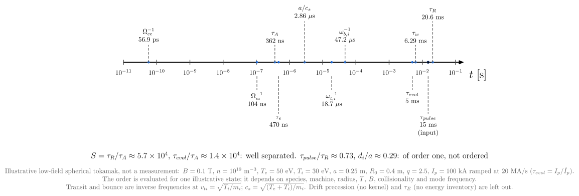
timescale_hierarchy evaluates the hierarchy of one illustrative low-field spherical-tokamak state rather
than assuming it. Every time comes from a formula kernel; only the pulse length is an input.
- Clearly ordered: $S$ and $\tau_{evol}/\tau_A$, both about $10^4$.
- Of order one, so not ordered:
- $\tau_{pulse}/\tau_R \approx 0.7$. Resistive relaxation has to be checked, not assumed either way. $\tau_R$ carries no geometric factor, and the slowest cylindrical mode decays $j_{01}^2 \approx 5.8$ times faster.
- $d_i/a \approx 0.3$, so Hall corrections are not globally negligible.
The axis also places the sound crossing time $a/c_s$ and the inverse thermal-ion transit and bounce
frequencies (#1739). They show where neoclassical and drift-kinetic dynamics sit between $\tau_A$ and the
evolution time. Drift precession has no formula kernel, and $\tau_E$ needs an energy inventory the state
does not carry, so neither is drawn. spatial_scale_orderings places the lengths of the same state on one
axis: the Larmor radii, $\rho_s$, $d_i$, the banana width, an illustrative gradient length, $a$, $R_0$ and
$qR_0$.
These numbers come from an illustrative state, not a measured discharge. Answering the same questions across the VEST database is the ordering atlas of #1629.
Ordering contracts
Whether an ordering holds depends on the model that assumes it. The contracts are registered in
vaft.validation.orderings.CONTRACTS as ApproximationContract objects of
vaft.validation.applicability (#1639). They are evaluated with evaluate_contract for one state and
evaluate_population for a table, whose columns are the names in ORDERING_QUANTITIES.
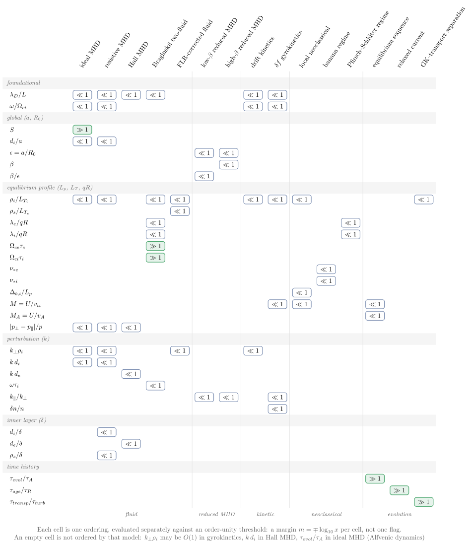
The quantities are grouped by the scale they are taken on, because the same ratio means different things on different scales. A global $d_i/a$, a mode’s $k\,d_i$ and a tearing layer’s $d_i/\delta$ are three rows: $d_i/a$ can be small while $d_i/\delta \sim 1$, and single-fluid MHD then fails in the layer.
| Group | Quantities |
|---|---|
| foundational | $\lambda_D/L$ (quasineutrality), $\omega/\Omega_{ci}$ (low frequency). They hold almost everywhere in a fusion core, so they rarely discriminate |
| global | $S$, $d_i/a$, $\epsilon = a/R_0$, $\beta$, $\beta/\epsilon$ |
| equilibrium profile | $\rho_i/L_{T_i}$, $\rho_s/L_{T_e}$, $\lambda_{e,i}/qR$, $\Omega_{ce}\tau_e$, $\Omega_{ci}\tau_i$, $\nu_{e}$, $\nu_{i}$, $\Delta_{b,i}/L_p$, $M = U/v_{ti}$, $M_A = U/v_A$, $\lvert p_\perp - p_\parallel\rvert/p$ |
| perturbation ($k$) | $k_\perp\rho_i$, $k\,d_i$, $k\,d_e$, $\omega\tau_i$, $k_\parallel/k_\perp$, $\delta n/n$ |
| inner layer ($\delta$) | $d_i/\delta$, $d_e/\delta$, $\rho_s/\delta$ |
| time history | $\tau_{evol}/\tau_A$, $\tau_{age}/\tau_R$, $\tau_{transp}/\tau_{turb}$ |
| Contract | Needs |
|---|---|
ideal_single_fluid_mhd |
$S \gg 1$; $d_i/a$, $k\,d_i$, $k_\perp\rho_i$, $\rho_i/L_{T_i}$, $\lvert p_\perp - p_\parallel\rvert/p \ll 1$; quasineutral and low frequency. Not $\tau_{evol}/\tau_A \gg 1$: ideal MHD describes Alfvénic dynamics, $\omega\tau_A \sim 1$ |
resistive_mhd |
the same without $S$, and with $d_i/\delta$, $\rho_s/\delta \ll 1$ in the layer it resolves. In a strong guide field $\rho_s$ is the layer’s two-fluid scale |
hall_mhd |
$k\,d_e$, $d_e/\delta \ll 1$; quasineutral. $k\,d_i$ and $d_i/\delta$ are not ordered: Hall MHD exists to keep them of order one |
braginskii_two_fluid |
$\lambda_{e,i}/qR \ll 1$, $\Omega_{ce}\tau_e$, $\Omega_{ci}\tau_i \gg 1$, $\rho_i/L_{T_i} \ll 1$, $\omega\tau_i \ll 1$; quasineutral |
flr_small_fluid |
$\rho_i/L_{T_i}$, $\rho_s/L_{T_e}$, $k_\perp\rho_i \ll 1$ |
low_beta_reduced_mhd |
$\epsilon$, $\beta/\epsilon$, $k_\parallel/k_\perp \ll 1$ ($\beta \sim \epsilon^2$) |
high_beta_reduced_mhd |
$\epsilon$, $\beta$, $k_\parallel/k_\perp \ll 1$ ($\beta \sim \epsilon$, so $\beta/\epsilon$ is not ordered) |
drift_kinetic |
$\rho_i/L_{T_i}$, $k_\perp\rho_i$, $\omega/\Omega_{ci} \ll 1$; quasineutral |
gyrokinetic_delta_f |
$\rho_i/L_{T_i}$, $k_\parallel/k_\perp$, $\omega/\Omega_{ci}$, $\delta n/n$, $M \ll 1$; quasineutral. $k_\perp\rho_i$ is not ordered, and that separates gyrokinetics from drift kinetics and MHD |
local_neoclassical |
$\rho_i/L_{T_i}$, $\Delta_{b,i}/L_p$, $M \ll 1$; fails in a pedestal or barrier |
banana_regime_neoclassical |
$\nu_{e}$, $\nu_{i} \ll 1$ |
pfirsch_schlueter_neoclassical |
$\lambda_{e,i}/qR \ll 1$, i.e. $\hat\nu \sim qR/\lambda \gg 1$ |
quasi_static_equilibrium |
$\tau_{evol}/\tau_A \gg 1$, $M$, $M_A \ll 1$ |
resistively_relaxed_current |
$\tau_{age}/\tau_R \gg 1$. An order-one value is ambiguous, because $\tau_R$ has no geometric factor |
gyrokinetic_transport_separation |
$\rho_i/L_{T_i} \ll 1$, $\tau_{transp}/\tau_{turb} \gg 1$ |
A contract lists only what its model requires. An empty cell means the model does not order that quantity, which is different from requiring it to be large. The parallel Knudsen number $\lambda/qR$, the inverse of $\hat\nu$ up to an order-one convention factor, is shared by the Braginskii closure and the Pfirsch–Schlüter regime: the collisional closure is the Pfirsch–Schlüter ordering, and it fails in the banana regime of a hot core. The reduced-MHD contracts list only the reduction’s own orderings, so evaluate them together with the ideal or resistive MHD contract.
Every threshold is order unity. The result is a continuous margin per ordering,
$m = \mp\log_{10}x$, and a status per contract (SUPPORTED, OUTSIDE, UNASSESSED, NOT_APPLICABLE),
never a single valid/invalid flag. A quantity a state does not carry is UNASSESSED, never a violation.
Signed ratios (Mach numbers, the pressure anisotropy) enter as magnitudes. An exactly zero value, as in a
static or isotropic state, has no logarithmic margin and is also UNASSESSED.
This covers the fluid-to-kinetic core of the hierarchy, not every subsidiary ordering of every derivation. Full Vlasov–Maxwell kinetics assumes none of these orderings and has no contract. A gyrofluid shares the gyrokinetic orderings and differs only in its closure. The plateau regime between banana and Pfirsch–Schlüter has no ordering of its own.
Ordering spaces and margins
Two orderings read together form an ordering space. Its lines are where an expansion parameter
reaches one. They are not empirical stability or operating boundaries. The spaces are registered in
vaft.validation.orderings.ORDERING_SPACES:
| Space | $x$ | $y$ | Reading |
|---|---|---|---|
resistive_two_fluid |
$d_i/a$ | $S$ | Hall / two-fluid separation against resistive separation |
closure_magnetization |
$\lambda_e/qR$ | $\Omega_{ce}\tau_e$ | local fluid closure against strong magnetization |
flr_collisional |
$\lambda_i/qR$ | $\rho_i/L_{T_i}$ | collisional fluid against FLR smallness |
flr_collisional_electron |
$\lambda_e/qR$ | $\rho_s/L_{T_e}$ | the same with electrons, for data without a trustworthy $T_i$ |
equilibrium_relaxation |
$\tau_{age}/\tau_R$ | $\tau_{evol}/\tau_A$ | resistive current relaxation against quasi-static equilibrium |
import pandas as pd
from vaft.process.ordering_state import ordering_table
from vaft.plot.ordering_space import ordering_space, ordering_margins_plot

# One row per state (illustrative VEST-like inputs); ordering_table adds the ordering columns.
inputs = pd.DataFrame({
    "a_m": [0.25, 0.25, 0.25], "r_geo_m": [0.45, 0.45, 0.45], "b_t_T": [0.15, 0.2, 0.25],
    "n_e_m3": [5e18, 1e19, 2e19], "t_e_eV": [20.0, 50.0, 100.0], "z_eff": [2.0, 2.0, 2.0],
    "ln_lambda": [12.0, 12.0, 12.0], "beta_t": [0.01, 0.02, 0.03],
    "efit_quality": ["good", "good", "poor"],
})
states = ordering_table(inputs).join(inputs[["efit_quality"]])
# One row per flux-surface point, with the profile orderings.
points = pd.DataFrame({"rho_i_over_LTi": [0.02, 0.05, 0.2, 0.8]})

fig, ax = ordering_space(states, "resistive_two_fluid", group="efit_quality")
fig, ax = ordering_margins_plot(states, points)   # global orderings per state, profile ones per point
ordering_space draws a population on log axes. It shows:
- the order-unity line of each axis;
- the region where both orderings hold, shaded;
- dashed lines one and two decades into the permitted side;
- the four quadrants, named by the regime each side means.
A quadrant name describes only these two orderings. “Ideal, single-fluid” says nothing about the other orderings of the ideal-MHD contract. A row whose value is missing or not positive is counted as unassessed and left off, never placed at a guessed position.
ordering_margins_plot(states, points) shows, for each ordering, the margin $m = \mp\log_{10}(x/x_0)$ of
every state or point, its median, the fraction with $m > 0$ and the number assessed. A global or
time-history ordering is read from states, once per state. Any other ordering is read from points,
once per flux-surface point. So $n$ and the fraction match vaft.process.ordering_state.ordering_margins
on the same data. A row without one quantity is left out of that ordering only. Each ordering is drawn
against its contract threshold $x_0$ (ordering_threshold), which is order unity today. The background
bands are MARGIN_LABELS:
| Margin $m$ [decades] | Band |
|---|---|
| $m > 2$ | over 2 decades |
| $1 < m \le 2$ | 1-2 decades |
| $0 < m \le 1$ | 0-1 decade |
| $m \le 0$ | outside |
The bands name the scale separation. They are not an applicability status: that stays the two-sided
SUPPORTED / OUTSIDE of evaluate_contract, which has no “marginal” on purpose. A margin of exactly
zero, a quantity at its threshold, falls in “outside”, as it is OUTSIDE there. The continuous margin
is the result, and margin_label only names its band.
Which codes consume which contracts
A contract says what a model assumes. A run’s vaft.code.formalism.PlasmaFormalism record (#1727) says which
model the run used. vaft.validation.model_contracts joins the two (#1823).
Every mode with its record and its contracts is tabulated, generated from the registry, in Plasma models: a guide, §9.
contracts_for(formalism) maps a record to the contracts it consumes, as (contract, role) pairs. It reads
the record’s fields as they are. The role says how the assumption enters the calculation. It is not a
statement about how much of the plasma the assumption covers:
| Role | How the assumption enters | Example |
|---|---|---|
governing |
the model the calculation solves rests on it | DCON ideal, CGYRO, NEO, EFIT |
outer_solution, layer_solution |
it holds for the ideal outer solution, or for the resistive inner-layer solution, of a matched calculation | RDCON + RMATCH; STRIDE is outer_solution only |
fluid_part, kinetic_response |
it underlies a fluid energy principle, or the kinetic term added to it | DCON kinetic, GPEC kinetic |
closure |
it underlies a kinetic quantity evaluated on a given fluid displacement, not fed back | PENTRC |
inherited |
a reduced model is derived from a theory that rests on it, but does not solve that theory | TGLF, TGLF-NN (gyrokinetics); NEO’s analytic values |
transport_coupling |
local turbulent fluxes drive a transport solver | none yet (opt-in, see below) |
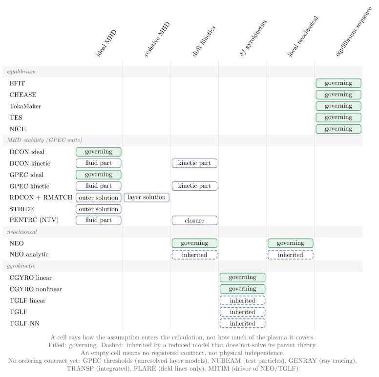
How to read the figure:
- The figure is deliberately simple. The validity conditions behind each cell are listed below, not drawn.
- An empty cell means no registered contract. It does not mean the calculation is independent of that
physics. A part of a formalism that no contract covers is returned as a reason, never as a guessed contract:
- test-particle orbit orderings (NUBEAM);
- full-$f$ gyrokinetics;
- a reduced model’s own closure or fit.
- Governing vs inherited. CGYRO solves gyrokinetics, so the gyrokinetic contract governs it. TGLF and TGLF-NN only inherit it. Their gyro-Landau-fluid closure, saturation rule and, for TGLF-NN, the training domain add assumptions that no ordering contract states. A gyrokinetic ordering that holds is therefore necessary for TGLF, not sufficient.
Validity conditions by mode. All modes are checked against the adapter code.
| Mode | Contracts and the conditions behind them |
|---|---|
| EFIT, CHEASE, TokaMaker, TES, NICE | equilibrium sequence: $\tau_{evol}/\tau_A \gg 1$, $M \ll 1$, $M_A \ll 1$. These are static force balance with scalar pressure, and make no claim about $S$, $k\,d_i$ or $k_\perp\rho_i$. |
| DCON ideal, GPEC ideal | ideal MHD governs: $S \gg 1$, $d_i/a$, $k\,d_i$, $k_\perp\rho_i$, $\rho_i/L_{T_i} \ll 1$, quasineutral, low frequency, scalar pressure |
| RDCON + RMATCH | ideal MHD for the outer solution; single-fluid resistive MHD (GGJ) for the inner layer, with $d_i/\delta \ll 1$ and $\rho_s/\delta \ll 1$. A large $S$ does not establish single-fluid validity in the layer. The layer width falls as a power of $S$: $\delta/a \propto S^{-2/5}$ for a $\Delta’$-driven tearing layer, and $S^{-1/3}$ for a resistive kink. So a larger $S$ makes the layer thinner and pushes $d_i/\delta$ and $\rho_s/\delta$ up. Two-fluid (drift-tearing) physics then enters even though the global ordering $S \gg 1$ holds better. The layer orderings are evaluated on $\delta$, never inferred from $S$. |
| STRIDE | the ideal outer solution and its $\Delta’$ only; no resistivity is solved. Its empty resistive-MHD cell is not independence from layer physics: reading $\Delta’>0$ as tearing-unstable passes through an inner-layer model STRIDE does not solve (constant-$\psi$, single-fluid), so the layer orderings of the RDCON row apply to that interpretation. |
| DCON kinetic, GPEC kinetic | ideal MHD for the fluid part; drift kinetics for the $\delta W_k$ term ($\omega/\Omega_{ci}$, $\rho_i/L$, $k_\perp\rho_i \ll 1$) |
| PENTRC | drift kinetics as a closure on a given ideal or kinetic GPEC displacement; the displacement’s own contract is the fluid part |
| NEO | drift kinetics and local neoclassical transport govern: $\rho_i/L$, $\Delta_b/L_p$, $M \ll 1$. All collisionality regimes are solved, so neither the banana nor the Pfirsch–Schlüter contract applies. |
| NEO analytic | the analytic, fitted and moment-method theory values a NEO run writes out (Hinton–Hazeltine, Chang–Hinton, Sauter, Redl, Hinton–Rosenbluth, NCLASS). They inherit the same contracts, plus each model’s own assumptions. |
| CGYRO linear, nonlinear | δf gyrokinetics governs: $\rho_i/L_{T_i}$, $k_\parallel/k_\perp$, $\omega/\Omega_{ci}$, $\delta n/n$, $M \ll 1$. $k_\perp\rho_i$ is not ordered. $M \ll 1$ is VAFT’s choice: its input writer sets MACH=0, while CGYRO itself supports sonic rotation. |
| TGLF linear, TGLF, TGLF-NN | gyrokinetics inherited: necessary, not sufficient (see above) |
Gyrokinetic–transport separation is opt-in. A standalone flux-tube run, linear or nonlinear, imposes a
fixed background. Comparing its fluxes with experiment still assumes $\tau_{transp}/\tau_{turb} \gg 1$. The δf
ordering makes turbulence-driven profile evolution $\rho_*^{-2}$ slower than the turbulence. It says nothing
about evolution driven by the current ramp or actuators, which dominates VEST’s ~10 ms discharges. The registry
books the separate contract only when the run’s fluxes drive a transport solver, as in a PORTALS-type
flux-matching loop (#1588, not yet in VAFT). This is a bookkeeping choice. The record has no
field that says so. A workflow therefore passes contracts_for(..., transport_coupled=True), or sets
AdapterMode.transport_coupled. No VAFT mode sets it today, so the figure has no coupling column.
Sources and checks:
ADAPTER_MODESlists the modes of VAFT’s adapters with their formalisms, from the audit in Plasma models.- CGYRO’s two modes are the records its own
plasma_formalismbuilds. - A test checks the GPEC-suite modes field by field against the records
vaft.code.gpecresolves from the packaged namelists. - Modes VAFT does not run are not listed. RDCON’s RPEC path is one:
rdcon.insetscoil%rpec_flag=f, even though the resolver can classify it. - The modes the audit leaves unresolved, today the GPEC threshold layer models, are listed with no record and a reason.
- Every physics adapter in
vaft/codehas a mode. A test enforces this. FLARE traces field lines through a given equilibrium and perturbation, and solves no plasma model. MITIM is a driver: the NEO and TGLF runs it launches are those modes, and its PORTALS loop (#1588) will be the firsttransport_coupledworkflow. Both are listed with a reason and no record.
advisory_ordering_check(formalism, state, points) evaluates those contracts on a run’s input:
stateis the global and time-history quantities ofvaft.process.ordering_state;pointsis its profile quantities.
A contract with a local ordering is evaluated at every point, and the most constraining point is reported. Each
result goes through evaluate_contract and is placed on the credibility applicability axis with
as_evidence. The statuses are the four of applicability, with no “marginal”. A quantity the input does not
carry is UNASSESSED, never a pass. This covers a mode’s $k_\perp\rho_i$ without mode numbers, and a layer
width. The check is advisory: it reports and never blocks a run.
Recorded in run provenance. ordering_provenance(formalism, state, points) reduces the check to a strict-JSON
record. It lists the contracts consumed with their roles, statuses, limiting orderings, margins and point counts.
A missing margin is null. Three adapters store it, one per family:
| Adapter | Where | State it adds itself | State a caller passes |
|---|---|---|---|
| EFIT | ordering_check in the resolved configuration: efit_configuration.json, EFITResult.configuration and each slice’s provenance |
none (EFIT’s inputs carry no $n_e$, $T_e$ or $\dot I_p$) | EFITConfig.ordering_state, e.g. from vaft.process.ordering_state |
| GPEC suite | GPECModuleRun.ordering_check of each prepared cell, carried by the asdict run manifest |
none | GPECSuiteConfig.ordering_state |
| CGYRO | CGYROResult.provenance["ordering_check"] |
$\rho_i/L_{T_i}$ and $\lambda_D/L_{T_e}$ from the local input (cgyro.local_ordering_state) |
run_cgyro(..., ordering_state=...): a mode’s frequency or $k_\parallel/k_\perp$, a measured flow |
The state is advisory. It never enters EFIT’s scientific identity and never changes a namelist or an input file.
A failure inside the check is recorded as an error entry; it never costs a run its result. For CGYRO, a finite
caller value takes precedence over a derived one, and a caller’s NaN does not hide it. If extra_parameters
override species keys (a gradient scan), nothing is derived from the staged input, and the record says why.
State keys that are not ordering quantities are listed under ignored.
Building the state from an ODS. vaft.process.ordering_state.ordering_inputs_from_ods(ods, t) returns
state, points and a provenance record for one equilibrium slice. It matches that slice to t, and the
core_profiles slice to the equilibrium, by time within 0.5 ms, never by index. $Z_{\rm eff}$ comes from the
caller or from the stored profile, never from an assumption; without it the resistive orderings stay
UNASSESSED. The plasma age needs the caller’s onset time. The kinetic EFIT chain passes
KineticEFITConfig.ordering_state to every PLASMA-scale run’s EFITConfig.
Not yet wired. No production workflow passes ordering_state yet, so a routine EFIT or GPEC record lists
the consumed contracts with every ordering UNASSESSED until its stage calls the builder (#1823).
CGYRO’s two local quantities are in GACODE’s units: $\rho_s$ is deuterium-normalised in $B_{unit}$. That is an
order-one difference from the local field, inside the order-unity thresholds.
Known gap. The drift-kinetic contract orders $\omega/\Omega_{ci}$ and $k_\perp\rho_i$. A steady
axisymmetric solve (NEO) or a zero-frequency one (DCON kinetic) has neither as an input, so that contract stays
UNASSESSED for those modes. A NaN at a profile point never hides a finite state value. The reported point is
the DataFrame’s index label when points is a DataFrame.
References
- S. I. Braginskii, in Reviews of Plasma Physics, Vol. 1, Consultants Bureau (1965), p. 205.
- J. D. Huba, NRL Plasma Formulary, Naval Research Laboratory (2019).
- D. Biskamp, Magnetic Reconnection in Plasmas, Cambridge University Press (2000).
- H. R. Strauss, Phys. Fluids 19 (1976) 134; Phys. Fluids 20 (1977) 1354.
- F. L. Hinton and R. D. Hazeltine, Rev. Mod. Phys. 48 (1976) 239.
- P. Helander and D. J. Sigmar, Collisional Transport in Magnetized Plasmas, Cambridge University Press (2002).
- E. A. Frieman and L. Chen, Phys. Fluids 25 (1982) 502.
- I. G. Abel et al., Rep. Prog. Phys. 76 (2013) 116201.
- F. I. Parra and P. J. Catto, Plasma Phys. Control. Fusion 52 (2010) 045004.
- R. D. Hazeltine and J. D. Meiss, Plasma Confinement, Dover (2003).
- K. V. Roberts and J. B. Taylor, Phys. Rev. Lett. 8 (1962) 197.