Data access and IMAS
vaft.machine_mapping is the layer that turns VEST machine reality — DAQ field codes, coil geometry
tables, digitizer CSVs, MATLAB exports — into an IMAS-compliant ODS. It is the only place in VAFT that
knows about VEST-specific things like “field code 102 is the Rogowski coil” or “PF2 changed height in 2025”.
Everything downstream (vaft.process,
vaft.formula, vaft.plot) consumes the ODS and never touches the raw
database.
flowchart LR
    SQL[(VEST SQL raw DB<br/>field codes)] --> MM
    GEO[Packaged geometry<br/>*.yaml / *.mat / *.csv] --> MM
    MAT[Thomson / CXRS<br/>.mat exports] --> MM
    CSV[SXR digitizer CSV] --> MM
    MM[vaft.machine_mapping] --> ODS[omas.ODS<br/>magnetics · tf · pf_active · ...]
    ODS --> DOWN[vaft.process / vaft.formula / EFIT / CHEASE]
If you only want to read already-mapped shots, you do not need this page — see Data structures. Read this page when you are mapping a new shot, adding a new diagnostic, or debugging why a mapped signal looks wrong.
The two-layer API
Every diagnostic module follows the same shape.
1. The canonical IDS entry point — named exactly after the IDS it fills. This is what you should call.
from vaft.machine_mapping.magnetics import magnetics
from vaft.machine_mapping.tf import tf

magnetics(ods, shot, tstart, tend, dt)   # fills ods['magnetics']
tf(ods, shot, tstart, tend, dt)          # fills ods['tf']
2. The vfit_* builders — the static/dynamic split underneath. *_static writes geometry and metadata
that do not depend on time; *_dynamic writes the time-dependent signals. The canonical entry point simply
calls both. Reach for these when you want geometry without touching the database, or want to re-map only the
waveforms.
from vaft.machine_mapping.tf import vfit_tf_static, vfit_tf_dynamic

vfit_tf_static(ods)                                  # tf.r0, ids_properties — no DB access
vfit_tf_dynamic(ods, shot, tstart, tend, dt)         # tf.coil.0.current, tf.b_field_tor_vacuum_r
All names are also re-exported lazily from the package root, so vaft.machine_mapping.vfit_md(...) works
without importing the submodule. The explicit from vaft.machine_mapping.<module> import <name> form used
above is what the production pipeline uses, and it is unambiguous — prefer it in scripts.
Coverage: which IDS, which module
| IDS | Module | Canonical entry point |
|---|---|---|
magnetics |
magnetics.py |
magnetics(ods, shot, tstart, tend, dt, processing_config=None) |
tf |
tf.py |
tf(ods, shot, tstart, tend, dt) |
pf_active |
pf_active.py |
pf_active(ods, shot, tstart, tend, dt, geometry_root=None) |
barometry |
barometry.py |
barometry(ods, shot, tstart, tend, dt) |
spectrometer_uv |
spectrometer_uv.py |
spectrometer_uv(ods, shot, t_start, t_end, dt) |
thomson_scattering |
thomson_scattering.py |
thomson_scattering(ods, shotnumber, data_root=None, mat_file=None) |
charge_exchange |
charge_exchange.py |
charge_exchange(ods, shotnumber, options='ces', data_root=None, mat_file=None) |
soft_x_rays |
soft_x_rays.py |
soft_x_rays(ods, shot, daq_label, **kwargs) |
dataset_description |
dataset_description.py |
dataset_description(ods, source, options=None) |
pf_passive |
pf_passive.py |
pf_passive(ods, source=None, options=None) |
em_coupling |
em_coupling.py |
em_coupling(ods, source=None, options=None) |
summary |
summary.py |
summary(ods, source, options=None) |
mhd_linear |
mhd_linear.py |
mhd_linear(ods, source, options=None) |
Note the argument shapes differ, and deliberately so — they follow the data source:
- Raw-DAQ diagnostics (
magnetics,tf,pf_active,barometry,spectrometer_uv) take(ods, shot, tstart, tend, dt): they resample DAQ traces onto a uniform window you choose. - File-backed diagnostics (
thomson_scattering,charge_exchange,soft_x_rays) take a shot plus a file/root override: their timebase comes from the exported file, not from you. - Reference-ODS diagnostics (
pf_passive,em_coupling) take asourcepath to a reference ODS.
equilibrium and pf_plasma exist as modules but their mapping functions raise NotImplementedError —
equilibria are produced by EFIT/CHEASE, not by machine mapping. See
Equilibrium.
Source: vaft/machine_mapping/
Mapping a shot end to end
This is the real production recipe, condensed from
generate_diagnostics_ods.py.
from omas import ODS, save_omas_json

from vaft.machine_mapping.dataset_description import dataset_description
from vaft.machine_mapping.magnetics import magnetics
from vaft.machine_mapping.pf_active import pf_active
from vaft.machine_mapping.spectrometer_uv import spectrometer_uv
from vaft.machine_mapping.barometry import barometry
from vaft.machine_mapping.tf import tf

shot, tstart, tend, dt = 39915, 0.26, 0.36, 4e-5

ods = ODS()
dataset_description(ods, shot, {"source_type": "shot", "run": 1, "machine": "VEST"})
pf_active(ods, shot, tstart, tend, dt)
spectrometer_uv(ods, shot, tstart, tend, dt)
barometry(ods, shot, tstart, tend, dt)
tf(ods, shot, tstart, tend, dt)
magnetics(ods, shot, tstart, tend, dt)

save_omas_json(ods, "39915_diagnostics.json")
Order matters only for dataset_description (it stamps the pulse/run identity). The rest are independent and
each writes into its own IDS.
dt = 4e-5 (25 kHz) matches the native DAQ rate — asking for a finer grid does not create information, it
just interpolates.
Per-diagnostic detail
magnetics
The heaviest module, and the one you are most likely to need to reason about.
vfit_magnetics_static(ods) writes probe and loop geometry from packaged YAML: position.r, position.z,
a probe length of 0.01 m, poloidal_angle of $3\pi/2$, and type.index = 2 (Mirnov). It also appends four
toroidal reference Mirnov channels at $r = 0.796$ m, $z = 0.02$ m spaced at
$\phi = 0,\ 2\pi/3,\ \pi,\ 4\pi/3$ — these are what make toroidal mode-number analysis possible.
vfit_magnetics_dynamic(ods, shot, tstart, tend, dt, processing_config=None) fills:
| Node | Notes |
|---|---|
magnetics.flux_loop.:.flux.data |
integrated loop signal, multiplied by $2\pi$ to give poloidal flux in Wb |
magnetics.b_field_pol_probe.:.field.data |
integrated probe signal, T |
magnetics.b_field_pol_probe.:.voltage.data |
raw un-integrated Mirnov voltage at native DAQ timebase |
magnetics.ip.0.data |
plasma current, A |
magnetics.diamagnetic_flux.0.data |
diamagnetic flux, Wb |
The raw voltage traces are written by vfit_mirnov_raw_dynamic(ods, shot) and kept on the acquisition
timebase, not the resampled one — fluctuation analysis needs the full bandwidth. See
fluctuation_diagnostics_analysis.ipynb.
Two lower-level helpers are worth knowing:
from vaft.machine_mapping.magnetics import vfit_md, vfit_plasma_current, vest_diamagnetic_flux

time, flux_loops, probes = vfit_md(39915)          # -> (ndarray, list[ndarray], list[ndarray])
time, ip = vfit_plasma_current(39915)              # -> (ndarray, ndarray), amps
time, dia = vest_diamagnetic_flux(39915, 0.30, 0.34)  # needs the plasma start/end window
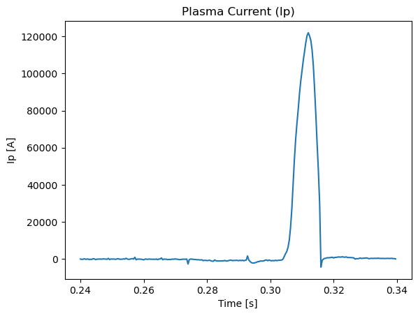
Plasma current is not just the Rogowski trace. The bare Rogowski signal picks up the vacuum-vessel and
coil contribution, so vfit_plasma_current subtracts a flux-loop-derived reference scaled by a mutual
inductance, then removes a linear baseline fitted on a pre-plasma window. The mutual inductance value and the
overall sign are both shot-range dependent (VEST rewired and re-polarised its diagnostics over the years),
which is exactly the kind of machine trivia this module exists to hide. If a historical shot’s $I_p$ comes out
inverted, that switch is the first thing to check.
Signal conditioning (integration, drift removal, smoothing) is delegated to vaft.process and is tunable
through processing_config, a VestMagneticsProcessingConfig:
from vaft.process.magnetics import VestMagneticsProcessingConfig
from vaft.machine_mapping.magnetics import magnetics

magnetics(ods, 39915, 0.26, 0.36, 4e-5,
          processing_config=VestMagneticsProcessingConfig())
See Signal processing for what those knobs do, and Magnetics for plotting the result.
tf
tf reconstructs the toroidal field from a Hall probe, not from a coil current shunt. The raw signal is
scaled by a Hall gain, baselined against the first samples, low-pass filtered and smoothed, then converted:
which is written to tf.b_field_tor_vacuum_r (units T·m). The VEST reference radius tf.r0 is 0.4 m, so
$B_t$ on axis is tf.b_field_tor_vacuum_r / tf.r0. The reconstructed coil current also lands in
tf.coil.0.current.
from vaft.machine_mapping.tf import vfit_tf_current, vfit_tf_bt_r

time, i_tf = vfit_tf_current(39915)   # A
time, bt_r = vfit_tf_bt_r(39915)      # T·m
pf_active
Ten PF coils. vfit_pf_active_static loads a discretized coil geometry MATLAB table and writes each coil
as a set of rectangular elements (geometry.geometry_type = 2) with turns_with_sign and area. Coil
resistance is computed from copper resistivity as
Crucially, which geometry file is loaded depends on the shot number — VEST’s PF set was modified, so
coil heights differ between the older and newer builds. Passing a shot to vfit_pf_active_static is what
selects the right one; the canonical pf_active(...) does this for you. You can point at a different asset
tree with geometry_root, and resolve a packaged asset directly:
from vaft.machine_mapping.pf_active import resolve_geometry_asset, vfit_pf

path = resolve_geometry_asset("VEST_DiscretizedCoilGeometry_Full_ver_2507.mat")
time, currents = vfit_pf(39915)   # currents: list of 10 arrays, A
Per-coil gains and noise reduction are applied while building the waveforms, so vfit_pf output is already
calibrated.
soft_x_rays
SXR does not come from the SQL DAQ — it comes from digitizer CSV files named
digitizer_{daq_label}_{shot}.csv. The mapper builds the timebase itself from a sample rate
(125 MHz / 128 by default) and a trigger offset, so daq_label is a required argument: it selects which
physical array the digitizer channels belong to.
from vaft.machine_mapping.soft_x_rays import soft_x_rays, soft_x_rays_from_digitizer_csv

soft_x_rays(ods, shot=39915, daq_label="22577", data_root="/path/to/sxr")

# or build a fresh ODS in one call
ods_sxr = soft_x_rays_from_digitizer_csv(39915, "22577", data_root="/path/to/sxr")
Line-of-sight geometry (channel.:.line_of_sight.first_point / .second_point) is filled from a packaged
endpoint table, and the default energy band is 0–20 keV. Channels the geometry table does not know about are
still stored as brightness traces, just without LOS metadata — so an unmapped channel degrades gracefully
rather than failing the run. Override the channel assignment with channel_map, and flip a mis-wired array
with polarity=-1.0.
Worked example:
soft_x_ray_signal_analysis.ipynb.
thomson_scattering and charge_exchange
Both read MATLAB exports rather than the DAQ, so they take a shotnumber and an optional data_root /
mat_file. Both write uncertainties alongside values when the export provides errors.
from vaft.machine_mapping.thomson_scattering import thomson_scattering
from vaft.machine_mapping.charge_exchange import charge_exchange

thomson_scattering(ods, 39915)                    # -> thomson_scattering.channel.:.{t_e, n_e}
charge_exchange(ods, 39915, options="ces")        # 'ces' or Doppler modes
charge_exchange supports more than one instrument: options selects between the CES export and the ion
Doppler spectroscopy exports, and read_doppler_single / read_doppler_profile are available if you want to
load Doppler data directly. These two IDSs are the kinetic input to profile fitting —
profile_fitting_using_equilibrium_and_kinetic_diagnostics.ipynb.
pf_passive and em_coupling
These two are not measured — they are machine constants. Both are copied from a packaged reference ODS that ships with VAFT:
from vaft.machine_mapping.pf_passive import pf_passive
from vaft.machine_mapping.em_coupling import em_coupling

pf_passive(ods)     # vessel/passive-loop geometry
em_coupling(ods)    # mutual inductance matrices
pf_passive deliberately deletes the loop currents and the time axis from the reference while keeping the
geometry. That is not a bug: the reference ODS contains one historical shot’s eddy currents, and you want the
geometry so you can compute your shot’s eddy currents fresh. Pass source (or options['reference_ods'])
to substitute your own reference.
em_coupling supplies the mutual inductances that eddy-current reconstruction needs; see
Signal processing and EM modeling.
dataset_description
Stamps pulse identity. vfit_dataset_description is the explicit form:
from vaft.machine_mapping.dataset_description import vfit_dataset_description

vfit_dataset_description(ods, shot=39915, run=0, machine="VEST", pulse_type="pulse")
# -> dataset_description.data_entry.{machine, pulse, pulse_type, run, user}
Static assets and the channel table
Machine mapping is only as good as its geometry tables. They live under vaft/data/geometry/ and are resolved
through resolve_data_root():
| Asset | Used for |
|---|---|
VEST_MagneticsGeometry_Full_ver_2302.yaml |
probe / flux-loop positions, and the inboard–side–outboard grouping |
MD.yaml |
magnetic-diagnostic channel list used by vfit_md |
table.yaml |
field code → channel name lookup |
VEST_DiscretizedCoilGeometry_Full_ver_1906.mat, ..._ver_2507.mat |
PF coil elements (shot-dependent) |
line_of_sight_endpoints.csv |
SXR lines of sight |
A separate vest.yaml shipped inside vaft/machine_mapping/ carries per-shot DAQ channel metadata (label,
field code, gain). It is keyed by shot, with a 0 block holding defaults that shot-specific blocks are
deep-merged over — so a recalibrated channel is a small YAML override, not a code change. Query it with:
from vaft.machine_mapping.utils import raw_database_info

info = raw_database_info("vest.yaml", 39915, "b_field_pol_probe")
info["labels"], info["fields"], info["gains"]   # dicts keyed by channel index
Probes and loops are grouped by position — inboard, side, outboard — and that grouping is what drives per-group uncertainties below.
Uncertainties for equilibrium reconstruction
EFIT needs an error bar on every constraint. machine_mapping attaches them, because the machine is what
determines them: an outboard Mirnov is not as trustworthy as a Rogowski coil.
from vaft.machine_mapping.utils import (
    DEFAULT_CONSTRAINT_UNCERTAINTIES,
    apply_default_constraint_uncertainties,
)

apply_default_constraint_uncertainties(ods)   # annotates pf_active, tf and magnetics in one call
The defaults are relative errors:
| Constraint key | Default |
|---|---|
pf_active_current |
1e-4 |
tf_b_field_tor_vacuum_r |
1e-4 |
magnetics_ip |
5e-2 |
magnetics_diamagnetic_flux |
3e-2 |
magnetics_bpol_inboard |
1e-2 |
magnetics_bpol_side |
1e-1 |
magnetics_bpol_outboard |
1e-2 |
magnetics_flux_loop_inboard |
1e-1 |
magnetics_flux_loop_outboard |
1e-2 |
The pattern is physical: coil currents are known to a part in $10^4$ because they are driven and metered, while the side probes and inboard flux loops get 10% — they sit where the field is weakest and the pickup worst, so down-weighting them is what keeps a reconstruction stable.
Override selectively with a mapping (unknown keys raise), or wholesale with a 9-element vector in the table’s order:
apply_default_constraint_uncertainties(ods, {"magnetics_ip": 0.02})
apply_default_constraint_uncertainties(ods, [1e-4, 1e-4, 2e-2, 3e-2, 1e-2, 1e-1, 1e-2, 1e-1, 1e-2])
Finer control is available per subsystem — apply_pf_active_current_uncertainties,
apply_tf_uncertainties, and apply_magnetics_uncertainties (which additionally accepts
fl_correct_coeff to divide out per-loop calibration coefficients). normalize_constraint_uncertainties
turns either input form into the canonical dict if you want to inspect it first.
Offline mapping and reproducibility
Live SQL access is not always available or desirable — CI, archived reprocessing, and anyone outside the VEST network need to work from a dump. Two environment variables control this, and the production pipeline sets both:
import os

os.environ["VAFT_RAW_SAMPLE_PATH"] = "/data/raw_dumps/39915.json.gz"
os.environ["VAFT_RAW_OFFLINE_ONLY"] = "1"     # never attempt a live SQL connection

# ... mapping calls now read from the dump
VAFT_RAW_SAMPLE_PATH accepts a {shot} placeholder, so one template serves a whole reprocessing campaign.
With VAFT_RAW_OFFLINE_ONLY set, a missing channel yields a zero waveform on a default timebase instead
of an exception — mapping completes and the gap is visible in the data rather than as a crash. When you see an
identically-zero trace in an offline run, suspect a missing channel in the dump before you suspect the machine.
Database access itself is documented in
vest_raw_signal_sql_database.ipynb.
Adding a new diagnostic
The contract to satisfy, in order:
- Create
vaft/machine_mapping/<ids_name>.py, named after the IMAS IDS, not the instrument. - Write
vfit_<ids>_static(ods, ...)for geometry/metadata andvfit_<ids>_dynamic(ods, shot, ...)for signals. Useset_pathfrom.utilsrather than assigning into the ODS directly — it keeps path handling uniform. - Write the canonical
<ids_name>(ods, shot, tstart, tend, dt)that calls both. - Put geometry in
vaft/data/geometry/as YAML or CSV. Do not hardcode positions in Python. - Register the public names in
_EXPORT_MAPand__all__in__init__.pyso they are reachable from the package root. - Degrade gracefully when a channel is absent — return an empty or zero signal, do not raise.
Related pages
- Quick start guide — load an already-mapped shot in five lines.
- Data structures — what an ODS/IDS is, and which IDSs VEST carries.
- Signal processing and EM modeling — the
vaft.processroutines that machine mapping calls into. - Magnetics — plotting the mapped magnetics IDS.
- Examples — the full notebook index.