VAFT API
This page is the map of the vaft package: what each subpackage is for, the entry points you are
expected to call, and where the detailed guide for each area lives. The signatures shown here are the
real ones — copy them.
import vaft

vaft.__version__          # '0.5.0' on the inspected develop baseline
Importing vaft is cheap. The top-level package exposes its subpackages lazily (__getattr__),
so import vaft does not drag in omas, imas or matplotlib until you actually touch
vaft.omas, vaft.imas or vaft.plot. Two compatibility shims are applied at import time —
vaft.apply_runtime_compat_patches() and vaft.apply_omfit_compat_patches() — which restore
NumPy/SciPy APIs that recent releases removed (trapz, cumtrapz, interp2d) so that OMFIT-derived
code keeps working. You never need to call them yourself.
Package map
flowchart TD
    RAW["VEST raw DAQ / SQL"] --> MM["vaft.machine_mapping<br/>raw signals to IMAS IDSs"]
    MM --> DB[("vaft.database<br/>load / save")]
    DB --> ODS["ODS / IDS<br/>(IMAS data model)"]
    ODS --> OMASL["vaft.omas<br/>ODS-aware find_ / compute_ / update_"]
    OMASL --> PROC["vaft.process<br/>signal and EM math"]
    OMASL --> FORM["vaft.formula<br/>closed-form physics"]
    ODS --> PLOT["vaft.plot<br/>figures"]
    ODS --> CODE["vaft.code<br/>EFIT / CHEASE / GPEC / TES"]
    CODE --> ODS
    ODS --> DATA["vaft.data<br/>GEQDSK I/O"]
    ODS --> IMASP["vaft.imas<br/>OMAS to IMAS Access Layer"]
| Subpackage | Purpose | Deep dive |
|---|---|---|
vaft.database |
Load/save VEST shots (ODS, native IDS) and reach the raw SQL DAQ archive | Data structures |
vaft.omas |
The ODS-aware API: find_*, compute_*, update_*, sample data |
this page |
vaft.process |
Array-in / array-out signal processing, EM response, magnetics chains | Signal processing and EM modeling |
vaft.formula |
Pure physics functions: equilibrium, stability, Green’s functions, constants | Formula reference |
vaft.machine_mapping |
Raw VEST DAQ to IMAS IDS mapping, plus uncertainty defaults | this page |
vaft.plot |
Matplotlib figures straight from an ODS/ODC | this page |
vaft.code |
Adapters for external codes (EFIT, CHEASE, GPEC, TES) | this page |
vaft.data |
GEQDSK read/write and packaged sample files | this page |
vaft.imas |
OMAS to IMAS Access Layer bridge | Data structures |
Everything in an ODS is in IMAS SI units: seconds, amperes, tesla, weber, m$^{-3}$, and eV or J
where the Data Dictionary says so. The plotting layer is the only place that rescales (for example A
to kA) and it does so through an explicit yunit argument.
vaft.database
The historical, and still the shortest, way to get a shot:
import vaft

ods = vaft.database.load(39915, source="public")        # eager omas.ODS
with vaft.database.open(39915, source="public") as remote:
    times = remote["equilibrium.time"]                   # lazy, read-only
load() returns an ODS unless representation="imas" is requested. paths scopes OMAS requests to
IDS roots or leaves; native requests accept top-level IDS names:
eq = vaft.database.load(
    39915, source="public", representation="imas", paths="equilibrium"
)
Full signatures:
vaft.database.load(shot, source="public", *, representation="omas", paths=None,
                   occurrence=None, imas_version=None, cache="auto", transport="auto")
vaft.database.open(shot, *, source="public", representation="omas", paths=None,
                   occurrence=None, imas_version=None)
vaft.database.save(data, shot, *, target="public", representation=None,
                   occurrence=None, imas_version=None, derived_cache="auto")
For local files use vaft.omas.load/save or vaft.imas.load/save; use
vaft.database.filedb.FileDB to resolve canonical archive paths. Remote save access is restricted and
is never required by the documentation examples.
Raw DAQ access
vaft.database.raw talks to the VEST SQL archive directly:
from vaft.database import raw

time, data = raw.vest_load(39915, field=109)     # (time_array, data_array), or None on failure
time, data = raw.load_raw(39915, fields=109)     # the loader vest_load delegates to
label      = raw.name(109)                       # field code to human-readable name
shots      = raw.vest_shots("2024-08-08")        # shots taken on a date
date       = raw.vest_date(39915)
latest     = raw.last_shot()
Other members worth knowing: raw.load_raw(shot, fields=None, daq_type=None, sample_opt=False)
(sample_opt points it at an archived dump instead of the live DB),
raw.vest_load_by_name(shot, name), raw.get_all_field_codes_for_shot(shot),
raw.dump_all_raw_signals_for_shot(shot, output_path=...) (offline cache) and its counterpart
raw.compare_db_and_dumped_raw_signals_for_shot(...). raw.sql_loading_available() and
raw.raw_offline_only() report whether the SQL driver and credentials are usable at all — this is
how the test suite decides to skip online tests. Credentials are managed by raw.setup_raw_db() and
raw.configuration() (backed by SecureConfigManager).
Connection and inventory helpers for the HSDS side live in vaft.database.utils:
from vaft.database import utils

utils.is_connect()                                   # is HSDS reachable?
utils.exist_shot(username=None, shot=None, data_filter=None, sort=-1)
vaft.omas
This is the layer you actually call to do physics on a shot. Everything here takes an ODS (or an
ODC) and reads/writes IMAS paths. It is a flat namespace: vaft.omas.<name> resolves into the
general, process_wrapper, formula_wrapper, update and sample modules.
Sample data (works offline)
ods = vaft.omas.sample_ods()    # packaged shot 39915
odc = vaft.omas.sample_odc()    # 39915, 41524, 41672
geq = vaft.omas.sample_gfile()  # packaged g-file as a GEQDSK object
Shot introspection — general
vaft.omas.find_shotnumber(ods)
vaft.omas.find_shotclass(ods, plot_opt=0)
vaft.omas.find_chamber_boundary(ods)
vaft.omas.find_breakdown_onset(ods)
vaft.omas.find_vloop_onset(ods)
vaft.omas.find_ip_onset(ods)
vaft.omas.find_pf_active_onset(ods)
vaft.omas.find_pulse_duration(ods)
vaft.omas.find_max_ip(ods)
vaft.omas.find_bt(ods)
vaft.omas.find_major_radius(ods)
vaft.omas.classify_shot(ods, pressure_threshold=0.01, halpha_threshold=0.01)
vaft.omas.print_info(ods, key_name=None)
vaft.omas.find_matching_time_indices(ods, time_slice=None, atol=1e-6)
Time-base bookkeeping (DAQ time versus breakdown-referenced time) and container plumbing:
vaft.omas.shift_time(one_ods, time_shift)
vaft.omas.change_time_convention(odc_or_ods, convention="vloop")
vaft.omas.odc_or_ods_check(odc_or_ods)     # returns an ODC either way
vaft.omas.combine_ods(ods_list)
Derived quantities — process_wrapper
These pull geometry and signals out of the ODS, call into vaft.process, and hand back arrays.
# Electromagnetic response and eddy currents
vaft.omas.compute_grid_ods(ods, xvar, zvar)
vaft.omas.compute_point_response_ods(ods, rz, plasma=None)
vaft.omas.compute_grid_response_ods(ods, plasma=None)
vaft.omas.compute_impedance_matrices_ods(ods, plasma)
vaft.omas.compute_eddy_currents(ods, plasma, ip, dt_sub=...)
vaft.omas.compute_point_vacuum_fields_ods(ods, rz=[(0.4, 0.0)], plot_opt=False, mode="vacuum")
vaft.omas.compute_null_ods(ods, time)

# Equilibrium, profiles, energy
vaft.omas.compute_core_profile_psi(ods, option="n_e", time_slice=None)
vaft.omas.compute_core_profile_2d(ods, option="n_e", time_slice=None)
vaft.omas.compute_magnetic_energy(ods, time_slice=None)
vaft.omas.compute_virial_equilibrium_quantities_ods(ods, time_slice=None)
vaft.omas.compute_volume_averaged_pressure(ods, time_slice=None, option="equilibrium")
vaft.omas.compute_reconstructed_diamagnetic_flux(ods, time_index=0)
vaft.omas.compute_diamagnetic_flux_measured_vs_computed(ods, time_slice=None)
vaft.omas.compute_diamagnetism(ods, time_index=0)
vaft.omas.compute_ohmic_heating_power_from_core_profiles(
    ods, time_slice=None, Z_eff=2.0, ln_Lambda=17.0)
Physics scalings — formula_wrapper
vaft.omas.compute_tau_E_exp(ods, time_slice, Z_eff=2.0)
vaft.omas.compute_tau_E_scaling(ods, time_slice, scaling="IBP98y2", Z_eff=2.0, M=1.0,
                                eng_params=None)
vaft.omas.compute_tau_E_engineering_parameters(ods, time_slice, Z_eff=2.0, M=1.0)
vaft.omas.compute_confiment_time_paramters(ods, time_slice, Z_eff=2.0, M=1.0)
vaft.omas.compute_power_balance(ods, include_line_radiation=True, line_radiation_species=None,
                                impurity_fractions=None, Z_eff=2.0)
vaft.omas.compute_bremsstrahlung_power(ods, time_slice=None, Z_eff=2.0)
vaft.omas.compute_voltage_consumption(ods, time_slice=None)
vaft.omas.compute_magnetic_shear(ods, time_slice)
In-place enrichment — update
update_* functions mutate the ODS: they fill IMAS fields that the reconstruction itself did not
provide. Run them once after loading, then plot.
vaft.omas.update_equilibrium_profiles_1d_normalized_psi(ods, time_slice=None)
vaft.omas.update_equilibrium_profiles_1d_radial_coordinates(ods, time_slice=None, plot_opt=0)
vaft.omas.update_equilibrium_boundary(ods, time_slice=None)
vaft.omas.update_equilibrium_coordinates(ods, time_slice=None, plot_opt=0)
vaft.omas.update_equilibrium_global_quantities_q_min(ods, time_slice=None)
vaft.omas.update_equilibrium_global_quantities_volume(ods, time_slice=None)
vaft.omas.update_equilibrium_profiles_2d_j_tor(ods, time_slice=None)
vaft.omas.update_equilibrium_profiles_2d_sfl_coordinates(
    ods, time_slice=None, profiles_2d_idx=1, convention="sfl", n_theta=129, plot_opt=0)
vaft.omas.update_equilibrium_stored_energy(ods, time_slice=None)
vaft.omas.update_equilibrium_constraints_diamagnetic_flux(ods, time_slice=None)
vaft.omas.update_core_profiles_global_quantities_volume_average(ods, time_slice=None)
vaft.process and vaft.formula
vaft.process is the numerical layer (NumPy in, NumPy out) and vaft.formula is the closed-form
physics layer. Neither one touches an ODS. Modules at a glance:
| Module | Contents |
|---|---|
vaft.process.signal_processing |
smooth, define_baseline, subtract_baseline, signal_on_offset, is_signal_active, process_signal |
vaft.process.numerical |
time_derivative(time, data) on a non-uniform grid |
vaft.process.electromagnetics |
compute_br_bz_phi, calc_grid, compute_response_matrix, compute_impedance_matrices, solve_eddy_currents, compute_vacuum_fields_1d |
vaft.process.magnetics |
rogowski_coil_ip, flux_loop_flux, b_field_pol_probe_field, mirnov_spectrogram, toroidal_mode_analysis, toroidal_phase_fit_at_time |
vaft.process.equilibrium |
psi_to_rz, psi_to_rho, volume_average, shafranov_integrals, efit_virial_volume_integrals, calculate_diamagnetism |
vaft.process.profile |
Thomson and charge-exchange mapping/fitting, core_profiles, core_profiles_from_eq |
vaft.process.statistical_analysis |
generate_core_profiles_history_dataframe, perform_ols_regression, compute_metrics |
vaft.formula.equilibrium |
flux, q and shear; geometry from an $(R,Z)$ boundary; virial (Shafranov) relations; power balance; confinement scalings |
vaft.formula.stability |
beta_N_from_beta_a_B0_Ip, greenwald_density, greenwald_fraction, ballooning/kink/sawtooth criteria |
vaft.formula.green |
greens_function_2d, green_br_bz, complete elliptic integrals |
vaft.formula.utils |
gradient, trapz_integral, fit_profile, make_fit_function |
vaft.formula.atomic |
interpolate_adf11, fractional_abundances, line_cooling_coefficient on OPEN-ADAS ADF11 tables |
vaft.formula.statistics |
residual, goodness-of-fit and convergence statistics (rms, chi_squared, runs_test_z, log10_decay_rate, …) |
vaft.formula.constants |
Physical constants used by the formula layer |
Both are documented in full on the Signal processing and EM modeling and Formula reference pages; the latter is generated per function from the standardized docstrings.
vaft.machine_mapping
This is how a raw VEST shot becomes IMAS. Each time-dependent diagnostic has a canonical function
with a uniform signature — (ods, shot, tstart, tend, dt) — that fills the corresponding IDS in
place:
import vaft
from omas import ODS

ods = ODS()
shot, tstart, tend, dt = 39915, 0.24, 0.36, 1e-4

vaft.machine_mapping.dataset_description(ods, shot)
vaft.machine_mapping.pf_active(ods, shot, tstart, tend, dt)
vaft.machine_mapping.tf(ods, shot, tstart, tend, dt)
vaft.machine_mapping.magnetics(ods, shot, tstart, tend, dt)
vaft.machine_mapping.barometry(ods, shot, tstart, tend, dt)
vaft.machine_mapping.spectrometer_uv(ods, shot, tstart, tend, dt)
Geometry, coupling and model IDSs take a source instead of a time window:
vaft.machine_mapping.pf_passive(ods)            # source=None uses the packaged geometry
vaft.machine_mapping.em_coupling(ods)           # packaged mutual-inductance matrices
vaft.machine_mapping.mhd_linear(ods, source)    # source = a linear-MHD output file
vaft.machine_mapping.summary(ods, source, options)
Two names in this namespace are reserved but not wired up yet:
vaft.machine_mapping.equilibrium and vaft.machine_mapping.pf_plasma raise
NotImplementedError. Equilibria enter the ODS through vaft.code (EFIT/CHEASE) instead.
Kinetic and imaging diagnostics take a shot number plus an optional data root:
vaft.machine_mapping.thomson_scattering(ods, shotnumber, data_root=None, mat_file=None)
vaft.machine_mapping.charge_exchange(ods, shotnumber, options="ces", data_root=None)
vaft.machine_mapping.soft_x_rays(ods, shot, daq_label, data_root=None, digitizer_file=None)
The *_from_raw_database variants — magnetics_from_raw_database, pf_active_from_raw_database,
tf_from_raw_database, barometry_from_raw_database, filterscope_from_raw_database,
dataset_description_from_raw_database, calculate_em_coupling_from_raw_database — are the
pipeline-facing entry points: they take an options dict and reach into the SQL DAQ themselves.
Per-channel entry points at that level (flux_loop_from_raw_database,
b_field_pol_probe_from_raw_database, rogowski_coil_and_ip_from_raw_database) exist as names but
raise NotImplementedError — use the IDS-level magnetics(...) mapping instead.
The vfit_* names are the legacy VEST-fit API, kept as aliases and split into
vfit_<diag>_static (geometry) and vfit_<diag>_dynamic (signals) — for example
vfit_magnetics_static / vfit_magnetics_dynamic, vfit_pf_active_static /
vfit_pf_active_dynamic, vfit_tf_static / vfit_tf_dynamic.
Uncertainties for equilibrium reconstruction are not hard-coded in the mapping; they come from a central table:
vaft.machine_mapping.DEFAULT_CONSTRAINT_UNCERTAINTIES       # dict
vaft.machine_mapping.DEFAULT_CONSTRAINT_UNCERTAINTY_VECTOR  # ordered vector

vaft.machine_mapping.apply_default_constraint_uncertainties(ods, uncertainty=None,
                                                            fl_correct_coeff=None)
vaft.machine_mapping.apply_magnetics_uncertainties(ods, ip_relative_error=None)
vaft.machine_mapping.apply_pf_active_current_uncertainties(ods, relative_error=None)
vaft.machine_mapping.apply_tf_uncertainties(ods, relative_error=None)
vaft.machine_mapping.normalize_constraint_uncertainties(uncertainty)
Geometry assets shipped with the package are resolved with
vaft.machine_mapping.resolve_geometry_asset(filename, geometry_root=None), and DAQ field metadata
with vaft.machine_mapping.raw_database_info(file, shot, key) and
vaft.machine_mapping.get_metadata(source).
vaft.plot
Every plotting function takes an ODS or an ODC (a multi-shot container) — pass an ODC and the shots
are overlaid. The common keywords are label ('shot', 'pulse', 'run', 'key', or an explicit
list), xunit ('s' or 'ms'), yunit, and xlim ('plasma', 'coil', 'none', or
[t0, t1]).
import vaft

ods = vaft.omas.sample_ods()

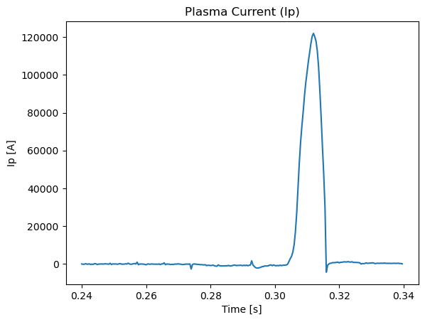
vaft.plot.time_magnetics_ip(ods, yunit="kA")
vaft.plot.time_pf_active_current(ods, indices="used", yunit="kA")
vaft.plot.time_magnetics_flux_loop_flux(ods, indices="all")
vaft.plot.time_magnetics_b_field_pol_probe_field(ods)
vaft.plot.time_tf_b_field_tor(ods)
vaft.plot.time_barometry_pressure(ods)
vaft.plot.time_spectrometer_uv_intensity(ods)
| Group | Functions |
|---|---|
| Time traces | time_magnetics_ip, time_magnetics_diamagnetic_flux, time_magnetics_flux_loop_flux, time_magnetics_flux_loop_voltage, time_magnetics_b_field_pol_probe_field, time_pf_active_current, time_pf_active_current_turns, time_tf_coil_current, time_tf_b_field_tor, time_tf_b_field_tor_vacuum_r, time_barometry_pressure, time_spectrometer_uv_intensity, time_impurity_effect, time_electromagnetics_current |
| Equilibrium scalars vs. time | time_equilibrium_plasma_current, time_equilibrium_li, time_equilibrium_beta_pol, time_equilibrium_beta_tor, time_equilibrium_beta_n, time_equilibrium_w_mhd, time_equilibrium_w_mag, time_equilibrium_w_tot, time_equilibrium_q0, time_equilibrium_q95, time_equilibrium_qa, time_equilibrium_major_radius |
| Energy and power | time_energy, time_beta, time_power_balance, time_voltage_consumption, time_virial_equilibrium_quantities |
| Profiles (1-D) | equilibrium_1d_radial, plot_onedim_profile, plot_onedim_profile_interactive |
| Geometry and 2-D | twodim_geometry_all, overlay_all, pf_passive_overlay, vacuum_psi_contour, overlay_all_with_vacuum_psi_contour, equilibrium_2d_profiles |
| Kinetic diagnostics | thomson_scattering_radial, thomson_scattering_time, thomson_scattering_radial_profiles, charge_exchange_radial, charge_exchange_time, charge_exchange_rho_profiles, plot_electron_psi_profile, plot_electron_2d_profile |
| Fluctuations | mirnov_signal, mirnov_spectrogram, toroidal_mode_spectrum, toroidal_phase_mode_fit |
| Soft X-rays | plot_soft_x_ray_los, plot_soft_x_ray_signal, plot_soft_x_ray_spectrogram, plot_soft_x_ray_pattern, plot_soft_x_ray_overview |
| Overviews | analysis_diagnostics, analysis_electromagnetics, time_equilibrium_analysis |
| Multi-shot history | plot_scaling_fit, plot_correlation_heatmap, plot_regression_summary, plot_tauE_exp_vs_scaling_loglog, plot_H_factor_distribution, plot_H_factor_vs_greenwald_fraction, confinement_time_exp_vs_scaling |
The Magnetics page shows several of these traces rendered from real shots.
vaft.code
Adapters for the external codes that VAFT drives. They all share one shape: a *Config (paths,
executable, run options), an *Inputs object produced by prepare_*, a run_* that executes the
code, and a collect_* / *Result pair that reads the outputs back.
When a configuration does not supply an executable explicitly, adapters follow the documented
installation roots: EFITHOME, CHEASEHOME, GPECHOME, and TESHOME. Missing binaries are a
readiness state, not a failure of deterministic input preparation.
from vaft.code import EFITConfig, prepare_efit_inputs, run_efit, collect_efit_outputs

cfg     = EFITConfig(...)
inputs  = prepare_efit_inputs(ods, cfg)      # k-file and constraint set
result  = run_efit(inputs, cfg)              # EFITResult
outputs = collect_efit_outputs(workdir, cfg)
| Code | Entry points |
|---|---|
| EFIT (equilibrium reconstruction) | EFITConfig, EFITInputs, EFITResult, prepare_efit_inputs, run_efit, collect_efit_outputs, generate_kfile, generate_constraints_ods, gfile_to_omas |
| CHEASE (fixed-boundary refinement) | CHEASEConfig, CHEASEInputs, CHEASEResult, find_chease_executable, prepare_chease_inputs, run_chease, refine_equilibrium |
| GPEC (perturbed equilibrium, 3-D response) | GPECSuiteConfig, GPECCaseInputs, GPECModuleRun, GPECSuiteResult, prepare_gpec_suite_case, run_gpec_suite_case, run_gpec, collect_gpec_suite_outputs, format_gfile_header_for_gpec |
| TES (forward equilibrium) | TESConfig, TESInputs, TESResult, prepare_tes_inputs, run_tes, collect_tes_outputs, scan_tes, parse_result_scalars, parse_result_coils |
| Base classes | CodeConfig, CodeInputs, CodeResult, CodeRunner |
refine_equilibrium(source, config=None) is the one-shot CHEASE convenience: g-file or ODS in,
refined equilibrium out. scan_tes(ods, base_config, values, param="ip0_kA") sweeps a single TES
parameter and collects every result. Snakemake rules should start with
vaft.code.init_snakemake_logger(snakemake) so that stdout and stderr land in the rule’s log file.
vaft.data
Portable file formats and the packaged sample files.
from vaft.data import read_geqdsk, write_geqdsk, to_omas, from_omas, sample_geqdsk, data_path

geq = read_geqdsk("g039915.00319")          # GEQDSK
ods = to_omas(geq)                          # GEQDSK to ODS (equilibrium IDS)
geq = from_omas(ods, time_index=0)          # ODS to GEQDSK
write_geqdsk(geq, "g039915.00319.copy")

geq  = sample_geqdsk()                      # packaged default: efit/g039915.00319
root = data_path()                          # the packaged vaft/data directory
from_imas and to_imas perform the same round trip against a native IMAS entry instead of an ODS.
vaft.imas
The OMAS to IMAS Access Layer bridge: load_omas_imas, save_omas_imas, imas_open,
imas_open_uri, imas_get, imas_set, plus IMAS_DD_VERSION_CONVERSION (the Data Dictionary
version used for conversion, overridable through the environment variable of the same name).
vaft.database uses this under the hood; call it directly only when you need to talk to an Access
Layer entry that is not a VEST shot. See
Data structures for worked examples.
Notebooks and workflows
Each subpackage has at least one notebook that exercises it end to end:
| Area | Notebook |
|---|---|
vaft.database |
database_initialization_and_load.ipynb |
vaft.database.raw |
vest_raw_signal_sql_database.ipynb |
vaft.data, vaft.imas |
imas_omas_data_conversion.ipynb, read_and_convert_data_structure.ipynb |
vaft.machine_mapping, vaft.process.magnetics |
magnetic_diagnostics_processing.ipynb |
vaft.process.electromagnetics |
electromagnetic_response_modeling_with_efund.ipynb, eddy_current_calculation_and_startup_analysis.ipynb |
vaft.code |
magnetic_equilibrium_reconstruction_with_efit.ipynb, equilibrium_refinement_using_chease.ipynb, perturbed_equilibrium_and_3d_response_with_gpec.ipynb, forward_equilibrium_using_TES.ipynb |
vaft.formula, vaft.process.statistical_analysis |
confinement_time_scaling.ipynb, tokamak_power_balance.ipynb |
vaft.plot |
plotting_sample_using_vaft_plot_module.ipynb |
The Snakemake pipelines that stitch these together live under
workflow/:
automatic_pipeline_1_routine_data_processing (raw DAQ to diagnostics ODS to constraints to EFIT and
CHEASE), automatic_pipeline_2_corrective_data_update (re-run equilibrium and profile updates on
existing shots), and automatic_pipeline_3_data_summary (multi-shot history tables and figures).
Source
Browse the package on GitHub: vaft/ —
database/,
omas/,
process/,
formula/,
machine_mapping/,
plot/,
code/,
data/,
imas/.
See also
- Quick start guide — install, connect, load a shot.
- Data structures — ODS, IDS and the IMAS data model.
- Signal processing and EM modeling —
vaft.processin depth. - Formula reference — every
vaft.formulafunction with definition, units, conventions and references. - Magnetics — plotting the magnetics IDS.
- Examples — the notebook index.