Particle motion: trajectories, invariants and animation

Compute once, select physical time

import numpy as np
import vaft.diagram as diagram
from vaft.process.particle import particle_motion_case
from vaft.plot import ParticleOrbitView, particle_overview

comparison = particle_motion_case("magnetic_mirror")
end = min(comparison.full.time[-1], comparison.guiding_center.time[-1])
times = np.linspace(0, end, 24)

# The scalar and animated calls select the same scientific state.
static = diagram.magnetic_mirror(trajectory=comparison, time=times[5])
movie = diagram.magnetic_mirror(
    trajectory=comparison, time=times, animation=True, fps=8
)
movie.save("mirror.gif")

s = np.linspace(-9.99, 9.99, 200)
view = ParticleOrbitView.from_comparison(
    comparison, bounce_coordinate=lambda x: x[2],
    well_coordinate=s, well_B=1 + (s / 10)**2,
)
fig, axes = particle_overview(view, time=times[5])
panels = particle_overview(view, time=times, animation=True, fps=8)

The mirror’s B(s) is stationary. Its marker, trajectory, velocity, energy partitions and invariant histories use the same physical timestamp. The renderer never re-integrates or recomputes diagnostics in a frame. Display-time interpolation is linear, recorded, and cannot extrapolate. The native Boris and adaptive GC sample times are retained independently of playback fps.

Supported experiments

particle_motion_case supports gyration, exb_drift, grad_b_drift, curvature_drift, toroidal_drift, magnetic_mirror, mirror_passing, tokamak_trapped, tokamak_passing and symmetry_breaking. Use charge=-1 to reverse charge-sensitive motion. Set aspect_ratio=1.5 for a qualified spherical-tokamak geometry reference; large-aspect-ratio banana scalings do not become accurate merely because that case can be integrated.

Default examples use an illustrative SI particle, q=1 C and m=1 kg. Resolved parameters are recorded. They are not electron/ion mass-ratio examples. speed, pitch_angle (radians), duration (seconds) and dt can be supplied. The benchmark helper rejects an initial abs(Omega_c)*dt > 0.3; inspect the maximum over the full orbit too and refine the step to establish accuracy.

The existing exb_drift, curvature_drift, toroidal_drift, guiding_center_invariants, canonical_toroidal_momentum, trapped_and_passing_orbits, toroidal_symmetry_breaking, ripple_well_formation and stochastic_ripple_orbit accept a computed trajectory, scalar/sequence time, and animation=True. Their historical calls without these controls keep their original static scenes. The computed extension shows one physical particle and its independently integrated GC; the historical two-species mass-ratio and schematic phase parameters belong to the static references. A replay through stochastic_ripple_orbit explicitly labels stochasticity as unestablished.

Reference animations

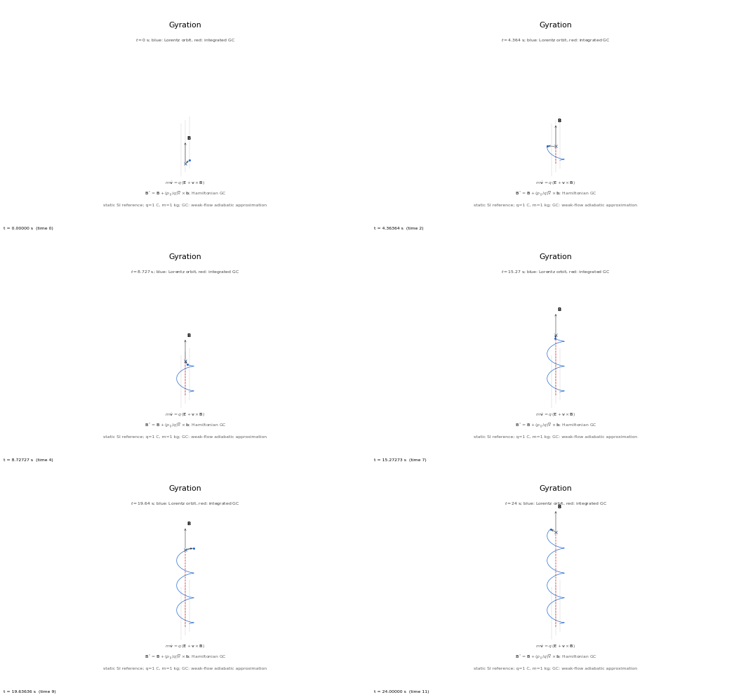
Cartesian gyration	Static magnetic mirror

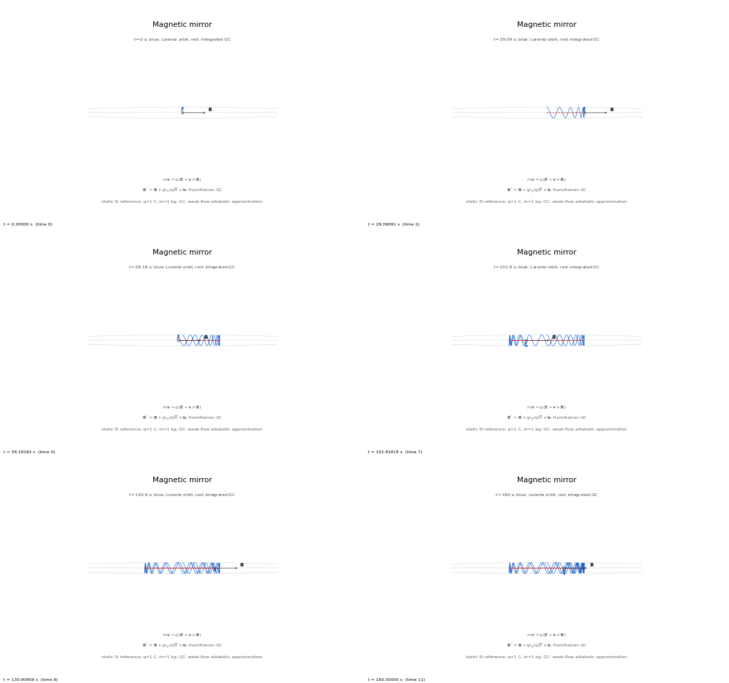The artifact manifest links all six families to animations and quantitative panels, and all but the tokamak and symmetry-breaking families to static SVGs. The mirror and invariants families share one experiment and so one panel image. The manifest also records the commit it was generated on and a SHA-256 of every scientific source its numbers depend on; the documentation catalog gate refuses a manifest whose sources have changed, and python -m workflow.particle_motion.run --check re-traces the six examples. Some manifest diagnostics are not meaningful for every family. orbit_class is no_resolved_turn for the cartesian and full-gc runs, which have no turning point to classify. gc_P_phi_residual_max is large for symmetry-breaking, because a 3-D field does not conserve P_phi; it is not a numerical error.

Physics and numerical contracts

vaft.data.particle.ParticleField uses right-handed Cartesian SI coordinates. A Jacobian has J[i,j] = dB_i/dx_j. Analytic derivatives are preferred; numerical derivatives require an explicit step and an h/h2 audit. An electrostatic field requires a consistent potential; potential gradients are checked. Domain queries precede field evaluation, including derivative probes.

vaft.process.particle exposes trace_particle_orbit, trace_guiding_center, particle_to_guiding_center, analyze_particle_orbit and compare_particle_orbits. The GC state is (X, p_parallel, mu) with mu held constant. The equations use B*=B+(p_parallel/q) curl(b) and the Hamiltonian H=p_parallel**2/(2m)+mu*B+q*Phi. DOP853 integrates scaled dimensionless states; position/momentum scales, tolerances and accepted times are recorded. It is not a symplectic method and has no long-time conservation guarantee.

GC validity requires magnetization and weak electric drift. Diagnostics report rho/L_B, parallel-curvature ordering, E×B speed/particle speed, and numerical steps relative to gyroperiod. The 0.1 educational warning threshold is recorded and is not a universal validity boundary. Full-orbit magnetic moment is an instantaneous drift-frame estimate; fixed GC mu is a model assumption. The initial particle/GC conversion is leading order and is not a first-order Lie transform. Comparison metadata distinguishes local-center subtraction from a centered one-gyroperiod time-window average with incomplete edges omitted.

Energy residuals use a kinetic/potential-variation scale. Canonical momentum residuals use mechanical/field contribution scales, preserving meaningful normalization even when the total initially vanishes. Canonical momentum uses an explicitly specified vector-potential gauge; the 3D example never substitutes an axisymmetric flux relation. Periods and toroidal precession are reported from completed bounce/transit intervals, with unwrapped angles.

Bounce action is defined only with a supplied signed periodic field-line arc coordinate. Incomplete cycles, unresolved closure and incorrect arc velocity are reported rather than assigned an action. The on-axis parabolic mirror has an exact harmonic period and action benchmark. Its field is exactly solenoidal and current-carrying; it is not an assumed vacuum-coil solution.

vaft.process.particle_fields provides uniform, slab, mirror and curl-defined toroidal/3D reference fields. equilibrium_particle_field reuses VAFT’s COCOS-aware equilibrium interpolator, preserving its documented F-edge clipping; its map is not extrapolated. filament_particle_field reuses the existing midpoint-rule Biot–Savart calculation and provides a vector potential with the same quadrature, plus a conductor exclusion region.

A trace returns its valid accepted prefix with an explicit reason for domain exit, field null, nonfinite field/state, unresolved derivatives, GC singularity, or integration failure. Initial data errors raise exceptions. Boundary termination is not a computed wall-impact location. At valid boundary samples, local energy and center diagnostics remain available even when the derivative stencil would cross the domain: derivative diagnostics are NaN, with a stencil_outside_domain audit. Comparison records incomplete derivative coverage and raises its ordering warning rather than certifying an unavailable estimate.

Steps smaller than the floating-point spacing of absolute timestamps are input errors. Shift t0 toward zero for short gyro-resolving intervals at a large time origin. Full-orbit updates advance by the represented timestamp interval.

Both diagram and diagnostic animation sidecars include full_orbit and guiding_center provenance records: charge, mass, initial state, field source, termination, integration method and solver settings. These records also cover custom comparisons created directly with the tracing APIs. Uniform-field provenance includes the supplied Cartesian B and E vectors. Straight background field lines follow the supplied uniform-field direction; arbitrary field geometries retain the sampled field arrow without invented straight lines.

Reproduction and limits

Run python -m workflow.particle_motion.run from the source root to generate six reference families, their GIFs, diagnostic panels, static SVGs (all but the tokamak and symmetry-breaking families) and artifact manifest under docs/assets/particle-motion/. Physical tests are in test/test_process_particle.py; replay tests are in test/test_particle_animation.py.

This implements the static-field portion of issues #2003–#2009. The slowly changing mirror experiment required by #2007 remains deferred, along with inductive/time-dependent fields, collisions, transport and external-solver cross-validation. The 3D reference is a controlled vacuum harmonic, not a calculated plasma response. Canonical-momentum change alone supports no claim of secular transport, stochasticity or NTV torque.