This branch contains 38 notebooks. The page inventories every one of them; the output cards below are published separately and are described under Verified notebook outputs.
How to read this index
The notebooks are at two different levels of maturity, and it saves a lot of time to know which is which before you open one:
Runnable — the notebook contains executable cells and a working data path. 27 notebooks.
Design shell — the notebook is currently a structured markdown outline (objectives, expected inputs and outputs, planned sections) with no code cells yet. 11 notebooks. They are useful as specifications of where a pipeline stage is heading, but they will not execute anything.
Design shells are marked (design shell) below.
Verified notebook outputs
The figures below were exported on 2026-08-21 with MPLBACKEND=Agg and VAFT_DOCS_READ_ONLY=1, from a commit and a branch that no longer exist, by an exporter that has since been removed from the repository. Every image still matches its recorded checksum, but none of them can be tied to the notebook that produced it, because the notebooks have moved on. They are kept as legacy artifacts and are labelled as such in _data/notebook_outputs.yml; regenerating them is tracked in issue #156. Treat them as illustrative, not as current output.
Offline first result
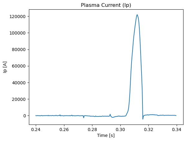
Plasma current from the packaged offline sample.Execution provenance
Inspect published-shot status and verify selected read paths without changing the remote namespace.
Start here. This is the shortest path from a fresh install to a shot in memory.
importvaft# Is the HSDS backend reachable?
print(vaft.database.is_connect())# Which shots are published?
shots=vaft.database.exist_shot("public")# Load one shot as an OMAS ODS
ods=vaft.database.load(39915,directory="public")
vaft.database.load is the canonical entry point: it returns an OMAS ODS, and it also accepts an explicit ids_name= keyword when you want a native IMAS IDS instead. See Database for the full surface.
If you have no network access, every example below can also be driven from the packaged sample data described in the next section.
Bridge OMAS ODS objects and native IMAS AL5 HDF5 storage, in both directions.
The packaged samples are the fastest way to get a realistic ODS without touching the network:
importvaftods=vaft.omas.sample_ods()# one shot
odc=vaft.omas.sample_odc()# a collection of three shots
list(ods.keys())print(ods["equilibrium.time"])print(list(ods["equilibrium.time_slice.0"].keys()))
To reach a packaged file by name rather than through the sample helpers, use the resource accessor — it resolves paths inside the installed package:
(design shell) Planned perturbed equilibrium and non-axisymmetric 3D response with GPEC.
CHEASE is the most complete code-coupling example in the repository. The prepare_* / run_* / collect_* triple is the pattern every code wrapper in vaft.code follows:
fromvaft.dataimportread_geqdskfromvaft.data.resourcesimportdata_pathfromvaft.code.cheaseimportCHEASEConfig,prepare_chease_inputs,find_chease_executableinitial=read_geqdsk(data_path("efit/g039915.00319"))ods=initial.to_omas()config=CHEASEConfig(workdir=workdir)inputs=prepare_chease_inputs(initial,config)# writes EXPEQ + chease_namelist
executable=find_chease_executable(config)# None if CHEASE is not installed
TES shows the same idea starting from a database shot rather than a file:
importvaftfromvaft.codeimporttesods=vaft.database.load(39915)cfg=tes.TESConfig(executable=RTES,workdir=WORKDIR,shot=39915,time=0.325,bt0=0.15,# fix the toroidal field; omit to read it from the tf IDS
eddy=True,# treat pf_passive as eddy coils
)inputs=tes.prepare_tes_inputs(ods,cfg)
Both binaries are optional: the notebooks degrade to input generation when the executable is absent. See Equilibrium and Stability.
(design shell) Planned cross-device comparison of geometry, equilibrium, and diagnostic signals.
The plot module names functions as {ids}_{coordinate}_{quantity} — for example time_magnetics_ip. Any plot function accepts a single ODS, an ODC, or a list of ODS objects, which is what makes shot overlays trivial:
importvaftods=vaft.omas.sample_ods()odc=vaft.omas.sample_odc()vaft.plot.time_magnetics_ip(ods)vaft.plot.time_magnetics_ip(odc)# overlays every shot in the collection
# Re-zero the time axis on breakdown, then replot
vaft.omas.change_time_convention(ods,convention="breakdown")vaft.plot.time_magnetics_ip(ods)
Deterministic stage and product summary for routine, corrective, and history-table Snakemake paths.
These pair with the automated Snakemake stages described in Pipelines.
Notebook maturity and remaining legacy APIs
The nine documentation-allowlisted notebooks are repaired on the companion branch. Some other runnable notebooks retained from the develop baseline still demonstrate older discovery or file-loading APIs; the working forms below are the migration path.
1. vaft.database.exist_ts_file() does not exist. It is called by tokamak_power_balance.ipynb and verification_and_validation.ipynb to discover processed shots. There is no replacement helper in the package; supply the shot list directly, as profile_fitting_using_equilibrium_and_kinetic_diagnostics.ipynb now does:
2. vaft.omas.load_omas_json() does not exist, and the packaged data moved. Sample JSON files are no longer flat under vaft/data/; they live under vaft/data/omas/. Notebooks that still build a path like os.path.join(os.path.dirname(vaft.__file__), "data", "39915.json") — including vest_daily_monitoring.ipynb and parts of read_and_convert_data_structure.ipynb — will fail. Use the sample helpers or the resource accessor instead:
importvaftfromvaft.data.resourcesimportdata_pathods=vaft.omas.sample_ods()# preferred
sample_path=data_path("omas/39915.json")# or resolve the file explicitly
Note that load_omas_jsondoes exist in the upstream omas package (from omas import load_omas_json); only the vaft.omas alias was removed.
Recommended order
A newcomer should work through the runnable notebooks in this order: