Experimental interpretation
The magnetics IDS is the backbone of every VEST analysis: it feeds the equilibrium reconstruction,
the eddy-current model, and all of the fluctuation diagnostics. This page shows what the IDS holds,
how VAFT builds it from raw DAQ signals, how the signals are conditioned, and how to plot each
quantity with the real vaft.plot API.
All figures below are shot #39915, which is also the ODS shipped inside the package
(vaft/data/omas/39915.json), so every snippet on this page runs offline.
What the IDS holds
| Node | VEST content |
|---|---|
magnetics.b_field_pol_probe.<i>.field.data |
64 $B_z$ pickup coils (integrated, calibrated, baseline-corrected) |
magnetics.b_field_pol_probe.<i>.voltage.data |
The same coils, raw un-integrated voltage at the native 250 kHz DAQ rate — this is the Mirnov signal |
magnetics.flux_loop.<i>.flux.data |
11 flux loops, in Wb |
magnetics.ip.0.data |
Plasma current from the Rogowski coil, flux-loop compensated |
magnetics.diamagnetic_flux.0.data |
Diamagnetic flux |
magnetics.time |
Common resampled time base for field, flux, ip, diamagnetic_flux |
Probes and loops are not grouped by an index list — VAFT classifies them geometrically at
runtime, from position.r / position.z:
| Group | Rule | Count in #39915 |
|---|---|---|
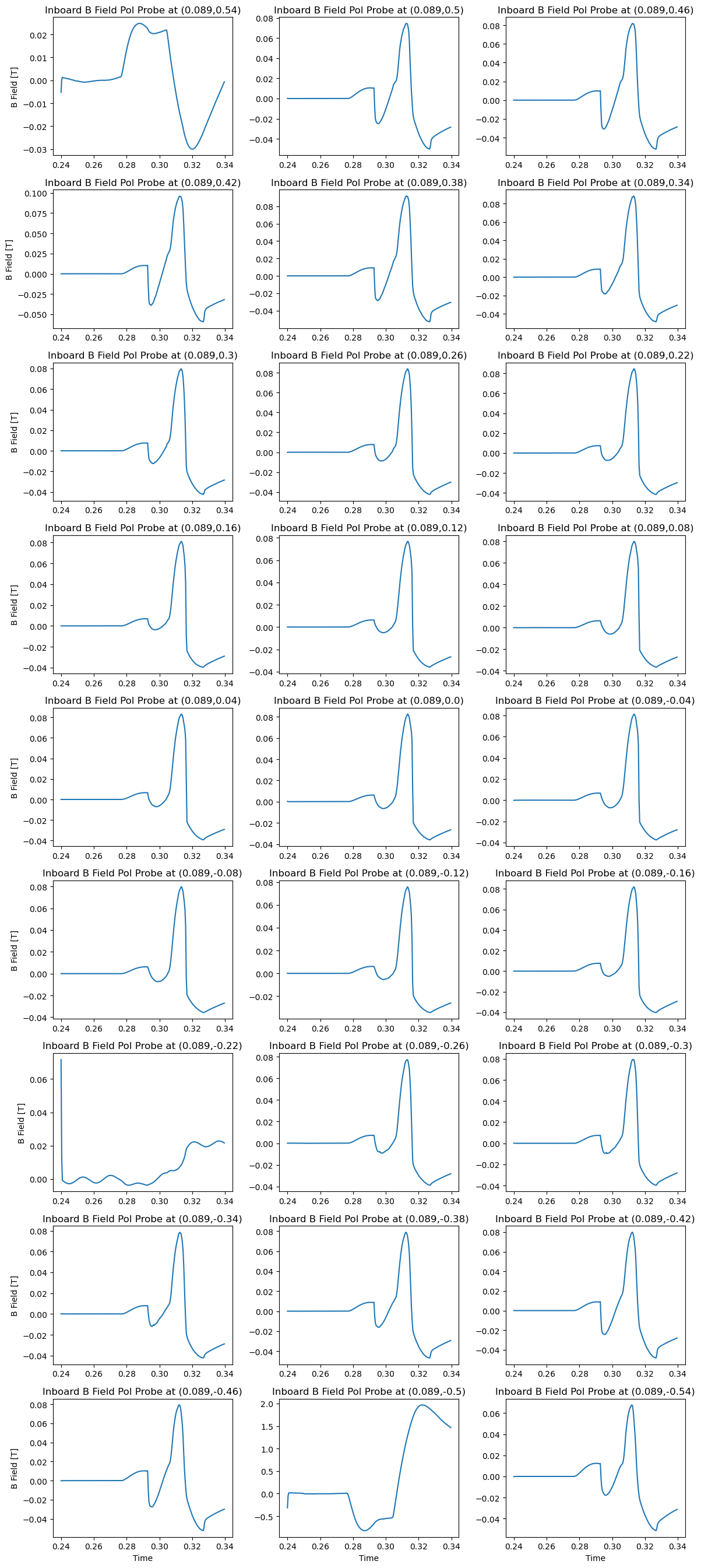
| Inboard $B_z$ probes | $r < 0.09$ m | 27 |
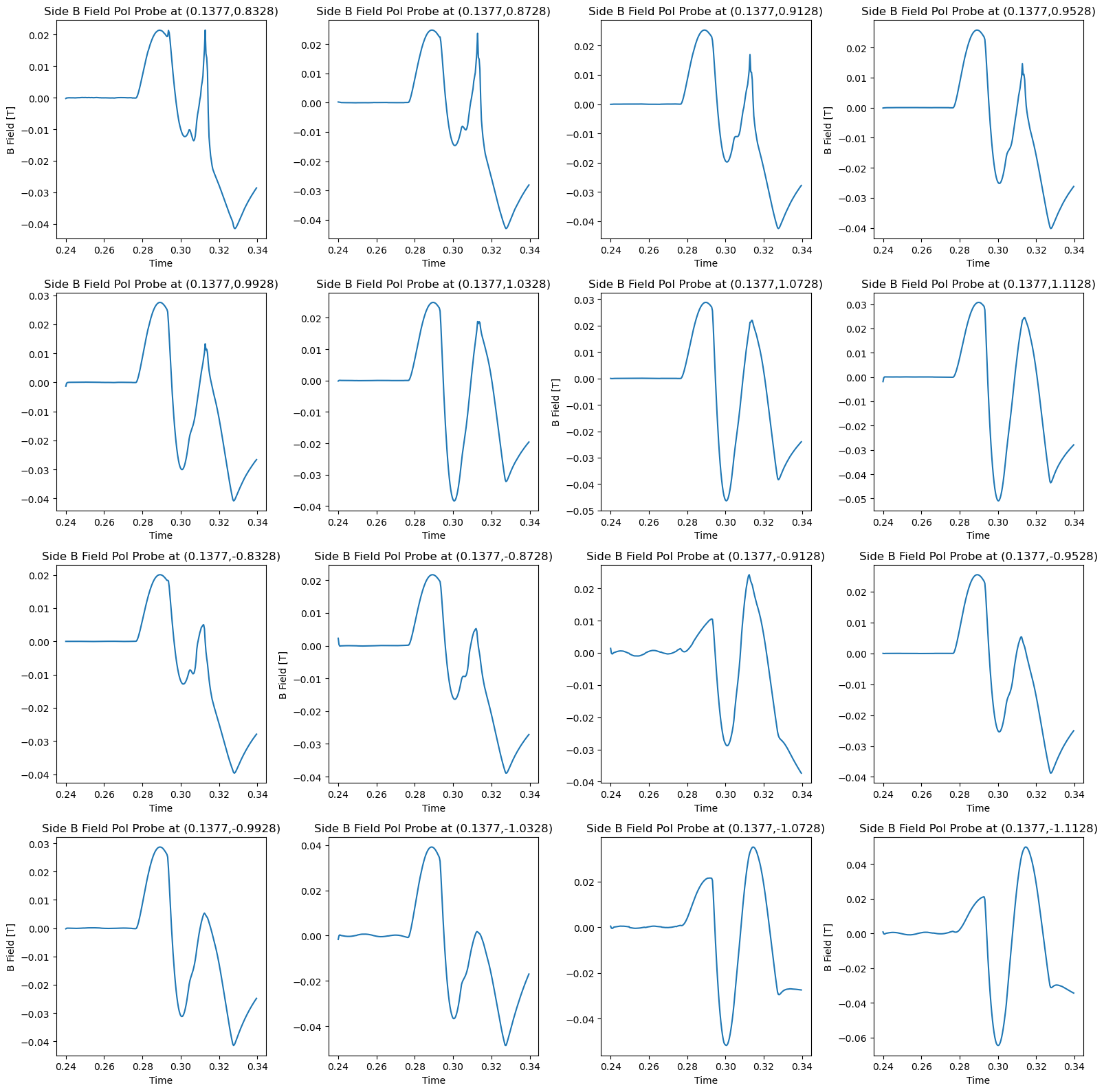
| Side $B_z$ probes | $|z| > 0.8$ m | 16 |
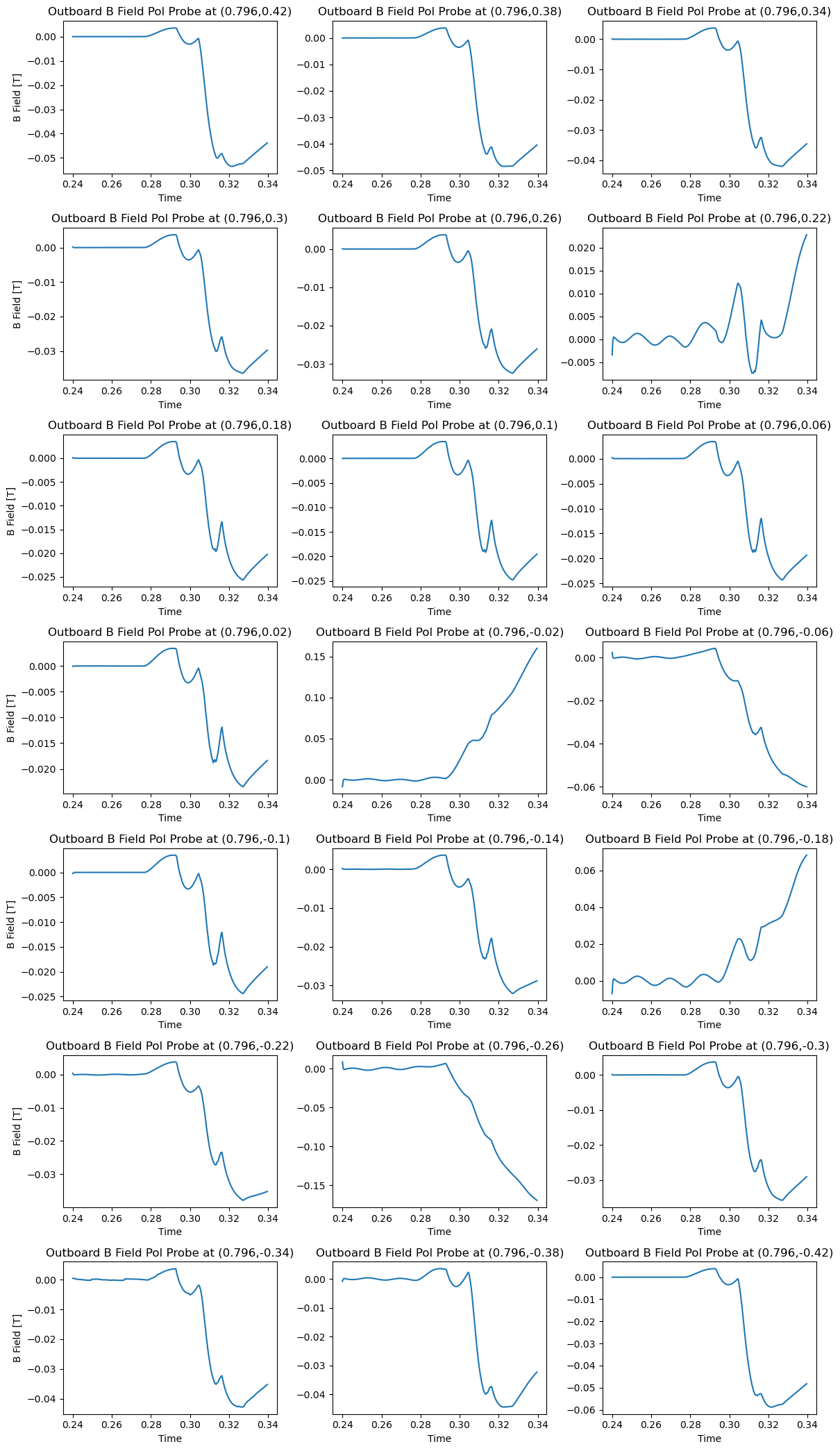
| Outboard $B_z$ probes | $r > 0.795$ m | 21 |
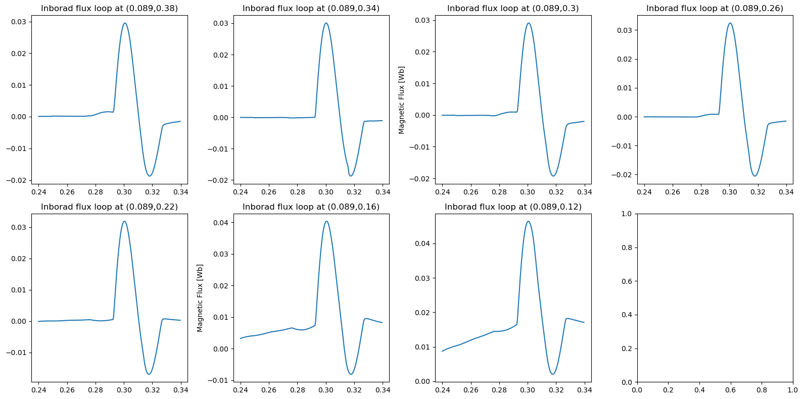
| Inboard flux loops | $r < 0.15$ m | 7 |
| Outboard flux loops | $r > 0.5$ m | 4 |
The same thresholds drive the indices= keyword of the plotting functions and the uncertainty
grouping in vaft.machine_mapping.apply_magnetics_uncertainties, so “inboard” means exactly the same
set of channels everywhere.
When a shot is mapped from raw signals, four extra toroidal Mirnov reference probes are appended after the 64 geometry probes (indices 64–67, at $\phi = 0, 2\pi/3, \pi, 4\pi/3$). They exist only to resolve toroidal mode numbers — see Mirnov and fluctuation diagnostics.
Loading a shot
import vaft

# Packaged sample — shot 39915, no database access, used by every example below
ods = vaft.omas.sample_ods()

# Or pull a shot from the VEST database
# ods = vaft.database.load_ods(39915, directory="public")

print(len(ods['magnetics.b_field_pol_probe']))   # 64
print(len(ods['magnetics.flux_loop']))           # 11
How the IDS is built
vaft.machine_mapping.magnetics is the only layer that knows about VEST field codes. It mutates the
ODS in place and returns None:
from omas import ODS
from vaft.machine_mapping.magnetics import magnetics

ods = ODS()
magnetics(ods, shot=39915, tstart=0.26, tend=0.36, dt=4e-5)
Underneath, magnetics is vfit_magnetics_for_shot, which runs a dynamic pass and a static
pass. You can call them separately — vfit_magnetics_static needs no shot and no database, so it is
the cheap way to get probe geometry:
from vaft.machine_mapping.magnetics import (
    vfit_magnetics_static,    # names, positions, angles from the geometry YAML
    vfit_magnetics_dynamic,   # time, field, flux, ip, diamagnetic_flux, raw Mirnov voltage
    vfit_mirnov_raw_dynamic,  # raw voltages only, at the native DAQ rate
)

vfit_magnetics_static(ods)
vfit_magnetics_dynamic(ods, 39915, 0.26, 0.36, 4e-5)
Raw signals consumed, by DAQ field code:
| Field code | Meaning |
|---|---|
| 102 | Rogowski coil (raw $I_p$) |
| 25 | Flux loop used to compensate the Rogowski mutual inductance |
| 101 | H-alpha — only used to find the discharge window for the diamagnetic baseline |
| 246 / 4 / 257 | Diamagnetic loop (the code is chosen by shot number) |
| 207, 241, 209, 171 | The four toroidal Mirnov reference probes |
Probe and flux-loop channels come from the packaged geometry tables
(vaft/data/geometry/VEST_MagneticsGeometry_Full_ver_2302.yaml, MD.yaml, table.yaml), not
from vest.yaml. Shot-number-dependent behaviour that silently changes results:
- Rogowski mutual inductance is
2.8e-4below shot 17455 and5.0e-4from 17455 on. - The $I_p$ sign is flipped for shot ≥ 20259.
- Flux-loop flux is written as
value * 2π(Wb, not Wb/rad).
If a raw signal is missing, these builders write zeros rather than raising. A fully populated,
entirely flat magnetics IDS is a symptom of a failed database read, not of a quiet shot.
To map a shot without a live database connection, point VAFT at an archived raw dump:
import os
os.environ["VAFT_RAW_SAMPLE_PATH"] = "vaft/data/legacy/shot_{shot}.json.gz"  # literal path or {shot} template
os.environ["VAFT_RAW_OFFLINE_ONLY"] = "1"
See Machine mapping for the full builder catalogue.
The processing chain
The physics kernels live in vaft.process and operate on plain NumPy arrays — no ODS. The whole VEST
magnetics chain is tuned by one frozen dataclass:
import vaft

cfg = vaft.process.DEFAULT_VEST_MAGNETICS_PROCESSING   # a VestMagneticsProcessingConfig
cfg.timebase()                     # 25 000 samples, 0 .. 0.99996 s
cfg.window_for_shot(39915)         # (6000, 8500, 8500)  -> index_start, index_end, baseline_end
cfg.window_for_shot(44740)         # (6500, 9000, 5000)  -> the "late" window

vaft.process.vest_magnetics_time_window(39915)   # the output time base for that shot
The window is shot-dependent: shots 41446–41451 and shots ≥ 41660 use the late window
(6500, 9000, 5000); everything else uses the default. Build your own config to override it:
from vaft.process.magnetics import VestMagneticsProcessingConfig
from vaft.machine_mapping.magnetics import magnetics

cfg = VestMagneticsProcessingConfig(lowpass_cutoff=5_000.0, sample_count=25_000)
magnetics(ods, 39915, 0.26, 0.36, 4e-5, processing_config=cfg)
The two per-channel kernels are deliberately not symmetric:
| Function | Chain |
|---|---|
vaft.process.vest_b_field_pol_probe_legacy(time, raw, calibration, *, shot, config=None) |
FIR low-pass (251 taps @ 2.5 kHz) → calibrate → negated cumulative-trapezoid integration → linear baseline subtraction |
vaft.process.vest_flux_loop_legacy(time, raw, calibration, *, flux_loop_number, config=None) |
calibrate → negated integration → divide by $2\pi$ → linear baseline subtraction. No low-pass. |
shot and flux_loop_number are keyword-only, and flux_loop_number is 1-based — the first flux
loop is 1, not 0. Loops 9, 10 and 11 get a different baseline window.
To run the whole batch yourself (this is what vfit_magnetics_dynamic calls):
time, flux_loops, probes = vaft.process.vest_md_signals(shot, channels, loader)
The lower-level building blocks are shared with every other diagnostic:
vaft.process.smooth, vaft.process.define_baseline, vaft.process.subtract_baseline
(fitting_opt ∈ 'linear', 'quadratic', 'spline', 'exp'), vaft.process.signal_on_offset,
vaft.process.time_derivative, and vaft.process.rogowski_coil_ip for $I_p$ from a Rogowski trace.
Details in Processing.
Measurement uncertainties
EFIT constraints need *_error_upper nodes. Write them with the relative errors VEST actually uses:
import vaft

vaft.machine_mapping.apply_magnetics_uncertainties(
    ods,
    ip_relative_error=0.05,
    diamagnetic_flux_relative_error=0.03,
    bpol_inboard_relative_error=0.01,
    bpol_side_relative_error=0.10,
    bpol_outboard_relative_error=0.01,
    flux_loop_inboard_relative_error=0.10,
    flux_loop_outboard_relative_error=0.01,
)

# Or the defaults for magnetics + pf_active + tf in one call:
vaft.machine_mapping.apply_default_constraint_uncertainties(ods)
All keywords are keyword-only. Channels that fall into none of the geometric groups get no uncertainty written at all.
Plotting
Every magnetics plotter takes an ODS or an ODC, calls plt.show(), and returns None. The shared
keywords are:
| Keyword | Values |
|---|---|
indices |
'all', a group name, an int, or a list of int |
label |
'shot' (default), 'run', 'key', or a list of one label per ODC entry |
xunit |
's' (default) or 'ms' |
yunit |
per function — see each section |
xlim |
'plasma' (default, the $I_p$ on/off window), 'coil', 'none', or [t0, t1] |
An invalid xlim or label prints a notice and falls back to the default; an invalid xunit/yunit
is silently ignored while the axis label still shows the unit you asked for. Don’t rely on
validation.
There is no time_slices argument on any magnetics plotter — a magnetics trace is a full time series.
To compare several shots, pass an ODC; that is the path that renders:
odc = vaft.omas.sample_odc()                       # shots 39915, 41524, 41672
vaft.plot.magnetics_time_ip(odc, yunit='kA', label='shot')
Both spellings of every name are live and equivalent: time_magnetics_ip (canonical) and
magnetics_time_ip (alias). The notebooks use the alias form.
Inboard $B_z$
27 pickup coils at $r < 0.09$ m, laid out on a 4 × 7 grid of subplots. Each panel title is the probe index and its $(r, z)$ position.
import vaft

ods = vaft.omas.sample_ods()          # shot 39915
vaft.plot.magnetics_time_b_field_pol_probe_field(ods, indices='inboard')
Outboard $B_z$
21 coils at $r > 0.795$ m, on a 3 × 7 grid.
vaft.plot.magnetics_time_b_field_pol_probe_field(
    ods, indices='outboard', xunit='ms', yunit='T', xlim='plasma'
)
Side $B_z$
| 16 coils at the upper and lower inboard corners, $ | z | > 0.8$ m, on a 4 × 4 grid. |
vaft.plot.magnetics_time_b_field_pol_probe_field(ods, indices='side')

# A single probe, or an explicit subset:
vaft.plot.magnetics_time_b_field_pol_probe_field(ods, indices=[4, 39])
Inboard flux loop
7 loops at $r < 0.15$ m, on a 2 × 4 grid. yunit='Wb'.
vaft.plot.magnetics_time_flux_loop_flux(ods, indices='inboard')
Outboard flux loop
4 loops at $r > 0.5$ m, on a 2 × 2 grid.
vaft.plot.magnetics_time_flux_loop_flux(ods, indices='outboard', xunit='ms')
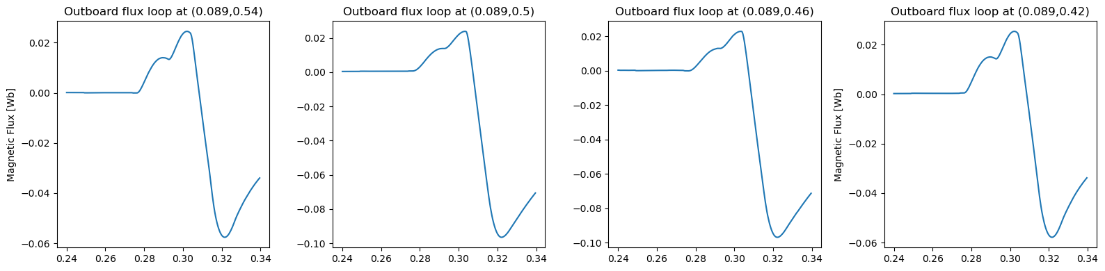
The loop voltage $V_{loop} = -\,d\Psi/dt$ is derived from the same flux data — the
inboard_midplane group ($r = 0.091$ m) is the one you want for the breakdown loop voltage:
vaft.plot.magnetics_time_flux_loop_voltage(ods, indices='inboard_midplane', yunit='V')
Plasma current
yunit accepts 'A', 'kA' and 'MA' (default 'MA').
vaft.plot.magnetics_time_ip(ods, yunit='kA', xunit='ms')
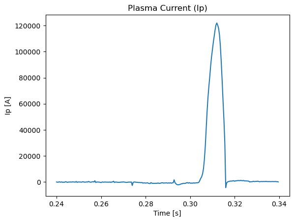
The default xlim='plasma' derives the window from the $I_p$ on/off times, so the discharge fills the
axes. Pass xlim='none' to see the full DAQ record, or xlim=[0.28, 0.34] for an explicit window.
Diamagnetic flux
vaft.plot.magnetics_time_diamagnetic_flux(ods, yunit='Wb')
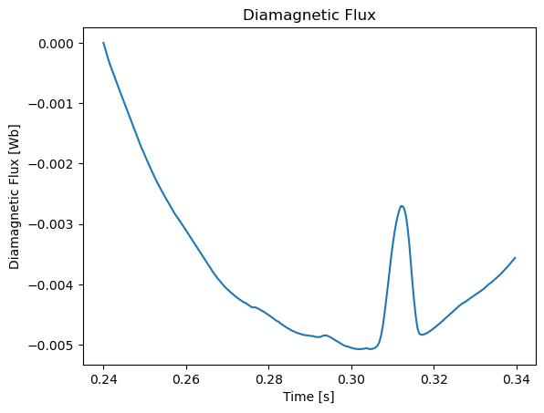
time_diamagnetic_flux is a different function: it overlays the raw magnetics flux with the
equilibrium-measured and equilibrium-reconstructed values, which is the check you want after an
equilibrium reconstruction:
vaft.plot.time_diamagnetic_flux(ods) # magnetics + equilibrium measured + reconstructed
See Equilibrium for how the reconstructed value is computed.
Mirnov and fluctuation diagnostics
The Mirnov analysis works on magnetics.b_field_pol_probe.<i>.voltage — the raw, un-integrated
coil voltage at the native 250 kHz DAQ rate. The packaged 39915 ODS carries only the integrated
field data, so build the ODS from a raw dump first (shot 44740 ships with the package):
import os
os.environ["VAFT_RAW_SAMPLE_PATH"] = "vaft/data/legacy/shot_{shot}.json.gz"
os.environ["VAFT_RAW_OFFLINE_ONLY"] = "1"

from omas import ODS
from vaft.machine_mapping.magnetics import vfit_magnetics_for_shot

ods = ODS()
vfit_magnetics_for_shot(ods, shot=44740, tstart=0.26, tend=0.34, dt=4e-5)
Unlike the older plotters, the Mirnov functions return (fig, ax) and accept ax= and
show=False, so they compose into your own subplot grid.
import vaft.plot as vplot

inboard_channel = 14
outboard_channel = 37
time_range = (0.304, 0.330)

fig, ax = vplot.mirnov_signal(
    ods,
    channels=[inboard_channel, outboard_channel],
    time_range=time_range,
    preprocess=True,          # False = raw volts; True = high-pass 2 kHz / low-pass 90 kHz, gain-corrected
    show=False,
)
ax.set_title("Mirnov voltage")
A spectrogram of one channel — max_frequency crops the frequency axis, window_size sets the FFT
window (must be even):
fig, ax = vplot.mirnov_spectrogram(
    ods,
    channel=inboard_channel,
    time_range=time_range,
    max_frequency=80e3,
    window_size=500,
    show=False,
)

# Ask for the numbers instead of just the picture:
fig, ax, result = vplot.mirnov_spectrogram(
    ods, channel=inboard_channel, time_range=time_range, show=False, return_result=True
)
result.time, result.frequency, result.magnitude    # a MirnovSpectrogramResult
Toroidal mode numbers
Two toroidally separated probes give the mode number $n$ from the cross-spectral phase,
$n = \arg\,S_{ab}(f) / \Delta\phi$. toroidal_mode_spectrum returns (fig, axes, result) with three
stacked panels (cross power, $n$, coherence):
import numpy as np

fig, axes, result = vplot.toroidal_mode_spectrum(
    ods,
    channel_pair=(65, 67),            # two of the four toroidal reference probes
    time_range=(0.304, 0.330),
    phase_geometry=np.pi / 6,         # toroidal separation of the pair, in radians
    show=False,
    return_result=True,
)
result.frequency, result.n, result.coherence       # a ToroidalModeResult
With all four probes you can fit the wrapped phase against toroidal angle at one instant and separate
several simultaneous modes. toroidal_phase_mode_fit returns (fig, ax, result):
fig, ax, fit = vplot.toroidal_phase_mode_fit(
    ods,
    center_time=0.310,
    channels=(64, 65, 66, 67),
    time_range=(0.304, 0.330),
    frequencies=[26e3, 52e3],         # None -> dominant peaks are picked automatically
    num_modes=2,
    candidate_n=range(0, 5),
    window_size=500,
    preprocess=True,
    show=False,
    return_result=True,
)
for mode in fit.modes:                 # sorted by amplitude, descending
    print(mode.frequency, mode.n, mode.rms_error)
Everything after * in these signatures is keyword-only, and the default channels (64–67) and pair
(65, 67) are the VEST toroidal reference probes — pass your own if you are analysing a different set.
The same kernels are callable without an ODS, on bare arrays:
import numpy as np
import vaft

time = np.asarray(ods['magnetics.b_field_pol_probe.14.voltage.time'])
data = np.asarray(ods['magnetics.b_field_pol_probe.14.voltage.data'])

clean = vaft.process.mirnov_preprocess_signal(
    data, sample_rate=250e3, high_pass_cutoff=2e3, low_pass_cutoff=90e3
)
spec = vaft.process.mirnov_spectrogram(
    time, clean, sample_rate=250e3, window_size=500, time_range=(0.304, 0.330)
)
print(spec.magnitude.shape)            # (n_frequency, n_time)

n_result = vaft.process.toroidal_mode_analysis(
    signal_a, signal_b, sample_rate=250e3, phase_geometry=np.pi / 6
)
Changing the time origin
t = 0 is the DAQ trigger by default. Every plot on this page can be re-referenced to the breakdown,
the loop-voltage onset, or the $I_p$ onset — the shift is applied to the ODS itself, so plot again
afterwards:
import vaft

ods = vaft.omas.sample_ods()
vaft.plot.magnetics_time_ip(ods)

vaft.omas.change_time_convention(ods, convention='breakdown')   # 'daq' | 'vloop' | 'ip' | 'breakdown'
vaft.plot.magnetics_time_ip(ods)
Notebook examples
- Examples — the full notebook index
plotting_sample_using_vaft_plot_module.ipynb— the canonicalvaft.plottourfluctuation_diagnostics_analysis.ipynb— the Mirnov / toroidal-mode workflow above, end to endvest_experimental_data_list.ipynb— what exists for which shot
Related pages: Machine mapping · Processing · Plotting · Data structures · Equilibrium · API reference
Credit : Hongsik-yun (peppertonic18@snu.ac.kr)