Electromagnetic modeling
vaft.process is the computation layer of VAFT. Almost every function in it takes plain NumPy
arrays and scalars and returns arrays, tuples or dataclasses — it does not read or write ODS. The
ODS-aware layer lives in vaft.omas (mainly vaft.omas.process_wrapper), which pulls geometry and
signals out of an ODS, calls into vaft.process, and writes the results back.
Rule of thumb:
vaft.processis the math,vaft.omas.compute_*is the API you usually call.
| Module | Concern |
|---|---|
vaft.process.signal_processing |
Smoothing, baseline definition/removal, filtering, on/off-set detection, liveness test |
vaft.process.numerical |
Time derivative on a non-uniform grid |
vaft.process.electromagnetics |
Green’s-function response matrices, R/L/M coupling matrices, eddy-current RL solve, vacuum-field reconstruction |
vaft.process.magnetics |
Legacy VEST EFIT magnetics chain, Mirnov preprocessing/spectrogram, toroidal mode numbers, Rogowski → $I_p$ |
vaft.process.equilibrium |
$\psi \leftrightarrow R \leftrightarrow \rho$ mapping, volume averages, diamagnetism, Shafranov/virial integrals |
vaft.process.profile |
Diagnostic→equilibrium mapping and profile fitting (writes core_profiles into ODS) |
vaft.process.statistical_analysis |
Log-log confinement-time scaling regression |
vaft/process/__init__.py is a star-import chain, so every public symbol below is reachable both as
vaft.process.<name> and as vaft.process.<module>.<name>. All of these work:
import vaft                                    # lazy: vaft.process is imported on first attribute access
from vaft.process import smooth
from vaft.process.magnetics import mirnov_spectrogram
Signal conditioning
Smoothing and de-spiking
import numpy as np
import vaft

ods = vaft.omas.sample_ods()                   # packaged VEST shot 39915
t   = np.asarray(ods['magnetics.time'])
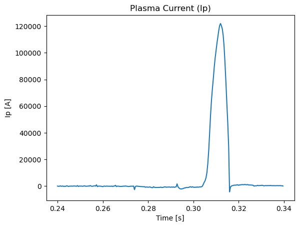
ip  = np.asarray(ods['magnetics.ip.0.data'])

ip_s = vaft.process.smooth(ip, 10)             # MATLAB-style moving average, edge-tapered
smooth(array, span) reproduces MATLAB’s smooth: the window narrows towards the two ends instead of
padding, an even span is decremented to the nearest odd value, and span <= 1 returns a copy. It is
1-D only and raises ValueError on anything else. It is the workhorse of the machine mapping layer
(pf_active, tf, magnetics all call it).
For PF coil-current traces there is a dedicated single-sample spike remover:
clean = vaft.process.vest_coil_current_noise_reduction(raw_coil_current)
It replaces sample $i$ with sample $i-1$ whenever $\lvert x_i \rvert - \lvert (x_{i+1}+x_{i-1})/2 \rvert > 0.001$. That threshold is hard-coded and absolute, so the trace must already be in the units the VEST coil digitizer produces.
Crop, resample, filter
process_signal is the general conditioning wrapper. Every key of the options dict is optional, and
they are applied in order (crop → resample → Butterworth filtfilt):
options = {
    'time_range': (0.27, 0.36),
    'resample': True,
    'dt': 4e-5,
    'filter_params': {'type': 'lowpass', 'cutoff': 1000, 'order': 4},
}
t_out, d_out = vaft.process.process_signal(t, ip, options)
type is one of 'lowpass', 'highpass', 'bandpass'; a bandpass requires cutoff=[low, high].
The sampling rate is derived as $1/(t_1-t_0)$, so the filter branch assumes a uniformly spaced time
base — resample first if it is not. Cutoffs are validated against Nyquist and raise ValueError when
out of range.
Two things about the order are worth being explicit about. The resample step goes through
resample_to_time (below), so reducing the sample rate anti-aliases on the input grid first. The
filter_params step that follows is a shaping filter, not an anti-alias filter, and its cutoff
is interpreted against the output grid’s rate.
Rate changes and anti-aliasing
VEST acquires on two DAQ rates — FAST_DT = 4e-6 (250 kHz) and SLOW_DT = 4e-5 (25 kHz), defined in
vaft/database/raw.py — while every processed time grid declared in
vaft/machine_mapping/vest.yaml is dt = 4.0e-5. A fast-DAQ channel written onto a policy grid is
therefore a 10× decimation.
This is the distinction the layer cares about:
- Interpolation evaluates a signal at new instants. Always fine.
- Downsampling reduces the sample rate. Content above the new Nyquist frequency does not disappear — it folds back into the band, where nothing downstream can tell it from real signal.
np.interp performs both and announces neither. Use resample_to_time instead anywhere a diagnostic
is written onto a common time grid:
from vaft.process import resample_to_time

intensity = resample_to_time(source_time, source_data, target_time)
resample_to_time measures both grids. When dt_target / dt_source is at or below min_ratio
(1.05) — alignment, an upsample, or a rate change too small to matter — it designs no filter and the
result is bit-for-bit np.interp. Above it, a zero-phase FIR low-pass runs on the source grid
before interpolating, with the passband edge at 0.8 × the target Nyquist by default (10 kHz for a
25 kHz grid): firwin sits at −6 dB at its cutoff and needs a transition band, so a passband edge
below Nyquist puts everything that can fold into the stopband.
firwin + filtfilt rather than resample_poly or decimate, for reasons specific to VEST.
resample_poly needs an exactly uniform source and an integer rational ratio; shots after 42190 store
linspace(0, span, n), so a nominally 4 µs grid is really 4.00016 µs, and the filterscope’s target
grid carries a legacy 0.24/0.26 s offset. Zero phase matters because filterscope intensity feeds onset
detection — a causal lfilter of the same design would move the onset by its group delay, about
0.66 ms or 16 target samples.
Where filtering would be wrong — a validity mask is logical, not bandlimited — pass
anti_alias=False. That is also exactly np.interp, so the decision shows up in the diff rather than
hiding in a numerical difference.
Two things it refuses rather than guesses at. A source grid that is not uniformly sampled raises
ResamplingError when a rate reduction is asked for: firwin/filtfilt assume even spacing, so on a
jittered grid the design rate is a fiction and the filter neither rejects what it should nor preserves
what it should. Resample onto a uniform grid first, or pass anti_alias=False to accept a bare
interpolation knowingly. And a source timebase that is not strictly increasing raises too, because
np.interp returns silent nonsense for an unsorted x — in this codebase that means the loader is
broken. (An unsorted target is fine: evaluating at scattered instants is exactly what interpolation
is for.)
Audit
Every time-domain rate change in vaft.machine_mapping and vaft.process, classified. Ratio is
dt_target / dt_source.
| Site | Source → target | Ratio | Classification |
|---|---|---|---|
machine_mapping/spectrometer_uv.py |
fields 138–144 fast 250 kHz → analysis 25 kHz |
10× | Was unfiltered; now resample_to_time |
machine_mapping/spectrometer_uv.py |
fields 101, 214 slow 25 kHz → 25 kHz | 1× | Pure alignment; unchanged output |
process/signal_processing.py (process_signal) |
arbitrary → dt |
any | Was resample-then-filter; now anti-aliased |
machine_mapping/langmuir_probes.py |
triple-probe solve → 25 kHz | ≤10× | n_e/te anti-aliased; solver_ok opts out (logical mask) |
machine_mapping/barometry.py |
gauge slow → full_discharge 25 kHz |
1× | medfilt is a de-spiker, not an anti-alias filter; routed through the primitive defensively |
plot/mirnov.py (_common_timebase) |
channel B → channel A’s grid | ≈1× | Routed through the primitive ahead of spectrogram/coherence |
machine_mapping/tf.py |
TF raw → full_discharge |
10× | Already safe: firwin low-pass on the source grid |
machine_mapping/pf_active.py |
PF raw → policy grid | 10× | Already safe: firwin + filtfilt |
process/magnetics.py |
probes/loops → 25 kHz | 10× | Already safe: firwin at 2.5 kHz on the 250 kHz grid |
machine_mapping/magnetics.py (FL10) |
250 kHz → decimated | 10× | Already safe: scipy.signal.decimate, order-8 Chebyshev I |
machine_mapping/impa.py |
IMPA raw → 25 kHz | ≤10× | impa_lowpass filters first, but the configured sample_rate may not match the channels (#425) |
process/electromagnetics.py |
EVD substepping | 1.25× | dt_sub ships coarser than the diagnostics grid — a solver-parameter bug, tracked separately |
code/efit/legacy.py |
4e-5 data on a 1e-4 ave_time step |
— | Pseudo-average, tracked separately |
process/profile.py, process/equilibrium.py, omas/update.py, omas/process_wrapper.py, code/*, formula/* |
ψ, ρ, R–Z grids; scalar sampling at one instant | — | Not time-domain rate changes; no action |
This table will rot. test/test_no_bare_downsample.py will not: it walks the AST of
vaft/machine_mapping and vaft/process and fails on any interpolation that neither goes through
resample_to_time nor carries an # anti-alias: comment recording which row above it belongs to.
Baselines
Baseline handling is a two-step API: build the index set of the “quiet” region, then fit and subtract a model over it.
idx = vaft.process.define_baseline(
    t,
    onset_time=0.28,        # seconds
    onset_window=500,       # number of SAMPLES before the onset index
    offset_time=0.34,       # seconds
    offset_window=100,      # number of SAMPLES after the offset index
)

corrected, baseline = vaft.process.subtract_baseline(t, ip, idx, fitting_opt='linear')
onset_time/offset_timeare times in seconds (converted internally withnp.searchsorted);onset_window/offset_windoware integer sample counts. Do not pass indices in the time slots.fitting_optaccepts'linear','quadratic','spline'(UnivariateSpline(s=0)) and'exp'; anything else raisesValueError.- The models are exposed for direct use with
scipy.optimize.curve_fit:linear_baseline(x, a, b),quadratic_baseline(x, a, b, c),exp_baseline(x, a, b, c). subtract_baselinereturns two arrays: the corrected signal and the fitted baseline.
Pulse window and channel liveness
onset, offset = vaft.process.signal_on_offset(t, ip, smooth_window=5, threshold=0.01)
t0, t1        = vaft.process.vfit_signal_start_end(t, ip, threshold=0.01)
alive         = vaft.process.is_signal_active(ip)          # -> bool
signal_on_offset applies a Savitzky–Golay smooth (polyorder 3) and returns the contiguous
above-threshold window containing the global maximum; vfit_signal_start_end does the same without
the smoothing stage. is_signal_active is a scale-invariant “is this channel alive?” test
(var_ratio_thresh=1e-2, change_ratio_thresh=1e-2) that returns False for arrays shorter than 2.
These are what the ODS-level event finders are built on — vaft.omas.find_breakdown_onset,
find_ip_onset, find_pf_active_onset and find_pulse_duration all call signal_on_offset
internally:
t_bd  = vaft.omas.find_breakdown_onset(ods)     # from the spectrometer_uv line intensity
t_dur = vaft.omas.find_pulse_duration(ods)
Deprecated aliases
Still live, still exported, but do not use them in new code:
| Alias | Canonical name |
|---|---|
VEST_CoilCurrentNoiseReduction |
vest_coil_current_noise_reduction |
vfit_signal_startend |
vfit_signal_start_end |
signal_onoffset |
signal_on_offset |
psi_to_RZ |
psi_to_rz |
Numerical helper
VEST time bases are not always uniform (a resampled or concatenated trace rarely is). Use
time_derivative rather than np.gradient when the spacing varies:
dip_dt = vaft.process.time_derivative(t, ip) # interval-weighted central difference
Forward difference at the first point, backward at the last, interval-weighted central difference in
between. It raises ValueError if the two arrays differ in shape or have fewer than two points.
Electromagnetic response (EFUND-style)
The response layer answers one question: what flux and field does a unit current in each conductor
produce at each observation point? Everything is built on the axisymmetric Green’s functions in
vaft.formula.green (green_br_bz for $B_R, B_Z$ and green_r for $\psi$, both per unit source
current), assembled into matrices that play the same role as EFUND’s response tables.
flowchart TD
    A["pf_active geometry<br/>pf_passive geometry"] --> B["compute_br_bz_phi<br/>one filament / obs points"]
    K["green_br_bz / green_r<br/>vaft.formula.green kernels"] --> B
    B --> C["compute_response_matrix<br/>sensors / arbitrary points"]
    B --> D["calc_grid<br/>regular R x Z grid"]
    E["em_coupling.mutual_passive_passive<br/>em_coupling.mutual_passive_active"] --> F["compute_impedance_matrices<br/>R, L, M"]
    F --> G["solve_eddy_currents"]
    C --> H["compute_vacuum_fields_1d<br/>psi, Br, Bz at points"]
    G --> H
    D --> I["null / vacuum psi contour"]
    G --> I
Single filament
br, bz, psi = vaft.process.compute_br_bz_phi(
    r_obs=np.array([0.4, 0.5]),
    z_obs=np.array([0.0, 0.0]),
    r_src=0.053,
    z_src=1.1924,
    shift=0.01,
)
shift is the desingularization knob: when an observation point falls within shift/3 of the
filament, the returned value is the average of the fields evaluated at $r_{\rm obs} \pm {\rm shift}$
instead of the divergent direct evaluation. Return order is (Br, Bz, Psi).
Response at sensors
compute_response_matrix evaluates the response at arbitrary $(r, z)$ points — diagnostic positions, a
radial line, a null-search stencil — and returns matrices of shape
(n_obs, nb_coil + nb_loop + nb_plasma):
Psi, Bz, Br = vaft.process.compute_response_matrix(
    observation_points=[[0.4, 0.0], [0.6, 0.0]],
    coil_data=[
        {'elements': [{'r': 0.053, 'z': 1.1924, 'turns': 4},
                      {'r': 0.053, 'z': 1.2124, 'turns': 4}]},
        # ... one dict per coil, 'elements' per turn-block
    ],
    passive_loop_data=[
        {'geometry_type': 1, 'outline_r': [0.30, 0.31, 0.31, 0.30],
                             'outline_z': [0.10, 0.10, 0.11, 0.11]},     # polygon
        {'geometry_type': 2, 'rectangle_r': 0.40, 'rectangle_z': 0.10},  # rectangle
    ],
    plasma_points=[[0.4, 0.0]],   # None / [r, z] / [[r1, z1], ...] are all accepted
)
The return order is (Psi, Bz, Br) — flux first. compute_response_vector is the same computation
with a different positional argument order. calc_grid, which builds the same physics on a regular
grid, returns (br, bz, phi) instead:
br, bz, phi = vaft.process.calc_grid(
    xvar, zvar,                                   # 1-D R and Z grid vectors
    coil_turns, coil_r, coil_z,                   # per-coil, per-element arrays
    loop_geometry_type, loop_outline_r, loop_outline_z,
    loop_rectangle_r, loop_rectangle_z,
)
# each output: (len(xvar)*len(zvar), nbcoil + nbloop), z varying fastest
calc_grid prints a running percentage to stdout every 100 grid points, and it takes the polygon
centroid of a geometry_type == 1 loop with a $1/(n-1)$ normalisation, whereas
compute_response_matrix uses a plain np.mean. The two therefore do not agree exactly for polygon
loops — do not mix them inside one workflow.
From an ODS
You do not normally build those dicts by hand. The ODS wrappers read pf_active and pf_passive
straight out of the data structure:
ods = vaft.omas.sample_ods()                             # 10 PF coils, 950 passive loops

Psi, Bz, Br = vaft.omas.compute_point_response_ods(ods, rz=[(0.4, 0.0), (0.6, 0.0)])
cpsi        = vaft.omas.compute_grid_response_ods(ods)   # (n_grid, nbcoil + nbloop)
compute_grid_response_ods uses the equilibrium.time_slice.0.profiles_2d.0.grid axes (dim1 = R,
dim2 = Z) as its observation grid, so an equilibrium IDS carrying a grid must be present.
Coupling matrices
The passive-structure circuit model needs three matrices:
\[R = \mathrm{diag}(R_w), \qquad M = M_{ww}, \qquad L = M_{wc}\]R from the per-loop resistances, M from the passive–passive mutual inductances, and L from the
passive–active mutuals (extended with plasma-filament columns when a plasma is present). The mutual
inductance matrices live in the em_coupling IDS (mutual_passive_passive, mutual_passive_active,
mutual_active_active) and can be populated from the packaged VEST reference with
vaft.machine_mapping.em_coupling(ods).
R_mat, L_mat, M_mat = vaft.omas.compute_impedance_matrices_ods(ods, plasma=[])
# R_mat: (nbloop, nbloop)   M_mat: (nbloop, nbloop)   L_mat: (nbloop, nbcoil [+ nbplas])
With plasma=[] the wrapper passes em_coupling.mutual_passive_active straight through (fast, and the
correct choice for a pure vacuum / startup study). With a non-empty plasma filament list, L is
recomputed from Green’s functions and the plasma columns are appended — expect a substantially
longer run time on the full 950-loop VEST vessel model. The matrices are also cached back into the ODS
under pf_passive['R_mat'], ['L_mat'] and ['M_mat'].
The underlying pure-array function is vaft.process.compute_impedance_matrices(loop_resistances,
passive_loop_geometry, coil_geometry, mutual_pp, mutual_pa, plasma_rz), where passive_loop_geometry
is a list of (loop_name, r_avg, z_avg, geometry_coef) tuples and coil_geometry is a list of
per-coil lists of (r, z, turns_with_sign).
Eddy currents and startup analysis
The circuit equation
The passive vessel currents $I_w$ obey
\[M \, \dot{I}_w + R \, I_w = -L \, \dot{I}_c\]where $I_c$ stacks the PF-coil currents and any plasma filament currents. solve_eddy_currents
integrates this with an eigenvalue decomposition of $A = -M^{-1}R$: the state-transition matrix
$E \, \mathrm{diag}(e^{\lambda \delta t}) \, E^{-1}$ is formed once, marched on a fine sub-step grid
(dt_sub, default $5 \times 10^{-5}$ s), then interpolated back onto the input time base.
I_w = vaft.process.solve_eddy_currents(
    R_mat, L_mat, M_mat,
    coil_plasma_currents,      # (n_times, nbcoil + nbplas)
    time,                      # (n_times,)
    dt_sub=5e-5,
)                              # -> (n_times, nbloop)
From an ODS
import numpy as np
import vaft

ods = vaft.omas.sample_ods()                       # VEST shot 39915

# Vacuum case: coils only, no plasma filament.
vaft.omas.compute_eddy_currents(ods, plasma=[], ip=[], dt_sub=5e-5)

print(np.asarray(ods['pf_passive.loop.0.current']).shape)   # (900,) — matches pf_active.time
To include the plasma as one or more current filaments, pass the filament positions and, for each of
them, a current trace on the pf_active time base:
t_pf = np.asarray(ods['pf_active.time'])
ip   = np.interp(t_pf,
                 np.asarray(ods['magnetics.time']),
                 np.asarray(ods['magnetics.ip.0.data']))

vaft.omas.compute_eddy_currents(ods, plasma=[(0.4, 0.0)], ip=[ip])
compute_eddy_currents calls compute_impedance_matrices_ods for you, solves the RL system, and writes
pf_passive.time plus pf_passive.loop.<i>.current back into the ODS.
Check the result.
solve_eddy_currentsdoes not raise on a singular $M$ or $R$: it falls backinv→pinv→ an array full ofnp.nan, after printing an error to stdout. Annp.isfinite(...).all()guard is worth the line.
Vacuum fields, loop voltage, decay index
Once the eddy currents exist, the vacuum flux and field at any set of points follow from the response matrices:
t, psi, br, bz = vaft.omas.compute_point_vacuum_fields_ods(
    ods,
    rz=[(0.4, 0.0)],
    mode='vacuum',       # 'vacuum' | 'pf_active' | 'pf_passive'
)
# psi, br, bz: (n_times, n_points)
mode selects which current sources contribute, which is exactly what separates the directly driven
field from the vessel’s response: 'pf_active' gives the coil-only field, 'pf_passive' the
eddy-current-only field, 'vacuum' their sum.
Differentiating the flux gives the loop voltage at that point (mind the $\psi$ convention of green_r
— flux per turn, not per radian — when comparing against a physical flux loop):
dpsi_dt = vaft.process.time_derivative(t, psi[:, 0])
v_loop  = -dpsi_dt
The field decay index $n = -\dfrac{R}{B_z}\dfrac{\partial B_z}{\partial R}$ — the quantity that decides whether a startup null is vertically stable — comes from the same call evaluated on a radial line:
r_line = np.linspace(0.25, 0.65, 41)
t, psi, br, bz = vaft.omas.compute_point_vacuum_fields_ods(
    ods, rz=[(float(r), 0.0) for r in r_line], mode='vacuum')

it      = int(np.argmin(np.abs(t - vaft.omas.find_breakdown_onset(ods))))
bz_line = bz[it]
n_index = -r_line * np.gradient(bz_line, r_line) / bz_line
The breakdown null
compute_null_ods contracts the grid response matrix with the coil and eddy currents at one time
and reshapes the result onto the equilibrium $(R, Z)$ mesh:
t_bd      = vaft.omas.find_breakdown_onset(ods)
psi, R, Z = vaft.omas.compute_null_ods(ods, t_bd)   # psi: (len(Zgrid), len(Rgrid))
Two ready-made figures follow exactly this path — a bare contour, and a contour over the machine geometry:
vaft.plot.vacuum_psi_contour(ods)                    # defaults to the breakdown onset time
vaft.plot.overlay_all_with_vacuum_psi_contour(ods)   # + coils, vessel, limiter, Thomson
Both mask $\psi$ to the chamber interior using vaft.omas.find_chamber_boundary(ods).
Magnetic diagnostics processing
The legacy VEST chain
The VEST EFIT input chain (FIR low-pass → calibration → negated integration → baseline subtraction) is reproduced exactly, with every magic constant lifted into one frozen dataclass:
from vaft.process.magnetics import (
    VestMagneticsProcessingConfig,
    DEFAULT_VEST_MAGNETICS_PROCESSING,
    vest_magnetics_time_window,
)

cfg = VestMagneticsProcessingConfig()              # 25 000 samples over 0 – 0.99996 s
cfg = VestMagneticsProcessingConfig(lowpass_cutoff=5_000.0, lowpass_taps=301)   # parameter scan

tb               = cfg.timebase()                  # (25000,)
i0, i1, base_end = cfg.window_for_shot(41660)      # -> (6500, 9000, 5000)
t_out            = vest_magnetics_time_window(41660, cfg)
window_for_shot is shot-dependent physics configuration, not a free tunable: shots 41446–41451 and
every shot ≥ 41660 use the “late” window (6500, 9000, 5000); everything else uses the default
(6000, 8500, 8500). Reprocessing a late shot with the default window silently changes the answer.
Per-channel entry points:
from vaft.process.magnetics import vest_b_field_pol_probe_legacy, vest_flux_loop_legacy

field = vest_b_field_pol_probe_legacy(time, raw, calibration, shot=39915, config=cfg)
flux  = vest_flux_loop_legacy(time, raw, calibration, flux_loop_number=1, config=cfg)
shotandflux_loop_numberare keyword-only.flux_loop_numberis 1-based. The config fieldflux_baseline_late_loop_numbers = (9, 10, 11)is matched against that 1-based number and selects a different baseline window for those loops.- The probe path low-passes (251-tap
firwinat 2.5 kHz); the flux-loop path does not, and divides by $2\pi$ whenflux_output_per_radianis true.
Batch processing over a channel table is vest_md_signals(shot, channels, loader, indices=None,
config=None), where channels is a sequence of dicts with keys field_code, calibration and kind
('flux_loop' or 'b_field_pol_probe'), and loader is any callable
(shot, field_code) -> (time, data) | None — returning None yields a zero-filled trace. VEST’s own
channel table and raw-database loader are already wired up in vaft.machine_mapping:
import vaft
from omas import ODS

time, flux_loops, probes = vaft.machine_mapping.vfit_md(39915)   # -> (time, list, list)

ods = ODS()
vaft.machine_mapping.magnetics(ods, shot=44740, tstart=0.26, tend=0.34, dt=4e-5)
Standalone processing chains
Three self-contained multi-channel routines exist for working outside the ODS:
from vaft.process.magnetics import rogowski_coil_ip, flux_loop_flux, b_field_pol_probe_field

t, ip = rogowski_coil_ip(time, rogowski_raw, flux_loop_raw,
                         flux_loop_gain=11, effective_vessel_res=5.8e-4,
                         baseline_type='linear', smooth_window=10)

t, flux, baselines = flux_loop_flux(time, raw, gain)            # raw: (m_samples, n_channels)

raw, filt, integrated, field, baselines = b_field_pol_probe_field(
    time, raw, gain, lowpass_param)                             # lowpass_param: FIR coefficients you design
rogowski_coil_ip subtracts a flux-loop reference from the Rogowski signal and auto-flips the sign
when $\lvert \min I_p \rvert > \lvert \max I_p \rvert$. Note the asymmetric returns:
b_field_pol_probe_field gives five arrays, flux_loop_flux gives three. Both accept
plot_opt=True, which builds an ipywidgets slider and so only does anything inside Jupyter.
Mirnov fluctuations and toroidal mode numbers
from vaft.process.magnetics import (
    mirnov_preprocess_signal, mirnov_spectrogram,
    toroidal_mode_analysis, toroidal_phase_fit_at_time,
)

clean = mirnov_preprocess_signal(data, sample_rate=250_000.0,
                                 high_pass_cutoff=2_000.0, low_pass_cutoff=90_000.0,
                                 amplifier_gain=1.0)            # all kwargs keyword-only

spec = mirnov_spectrogram(time, clean, sample_rate=250_000.0, window_size=500, time_resolution=1)
# spec.time, spec.frequency, spec.magnitude
mirnov_spectrogram is a manual Hann-window rFFT spectrogram (magnitude
$= 2 \lvert \mathrm{FFT} \rvert / N_{\rm win}$) that reproduces the legacy vest_mirnov.m.
window_size must be even and greater than 1.
Two-probe cross-spectral mode number, and multi-probe wrapped-phase fit:
res = toroidal_mode_analysis(signal_a, signal_b,
                             sample_rate=250_000.0,
                             phase_geometry=np.pi/6,          # toroidal separation [rad]
                             peak_threshold=0.1, sensor_count=4)
# res.frequency, res.n, res.power, res.phase, res.coherence, ...

fit = toroidal_phase_fit_at_time(time, signals, toroidal_angle,   # signals: (n_channels, n_time)
                                 center_time=0.3215,
                                 sample_rate=250_000.0,
                                 window_size=500,
                                 num_modes=2,
                                 candidate_n=range(-6, 7))
best = fit.modes[0]                                              # sorted by amplitude, descending
print(best.frequency, best.n, best.rms_error)
$n$ is recovered as $\arg \mathrm{CSD}(a,b) / \Delta\phi$, peak-picked on $\lvert \mathrm{CSD} \rvert$ and filtered by a coherence threshold. The plot module wraps all of this against an ODS — this is the path the fluctuation notebook takes on shot 44740:
import vaft.plot as vplot

vplot.mirnov_signal(ods, channels=[14, 37], time_range=(0.304, 0.330), preprocess=False)
vplot.mirnov_spectrogram(ods, channel=14, time_range=(0.304, 0.330), max_frequency=80e3)
vplot.toroidal_mode_spectrum(ods, channel_pair=(14, 37), time_range=(0.304, 0.330))

fig, ax, phase_fit = vplot.toroidal_phase_mode_fit(
    ods, center_time=0.3215, channels=[64, 65, 66, 67], return_result=True)
Statistical analysis
vaft.process.statistical_analysis fits a log-log power-law scaling
$\tau_E \propto \prod_k x_k^{\alpha_k}$ by ordinary least squares.
from vaft.process import statistical_analysis

df = statistical_analysis.load_data_from_excel(str(excel_file))
df = statistical_analysis.filter_dataframe(df)          # drops Ploss_MW > 3, takes abs(Bt_T)

eng_params   = ['Ip_MA', 'Bt_T', 'Ploss_MW', 'ne_19m3', 'R_m', 'epsilon', 'kappa']
target_param = 'tauE_s'

statistical_analysis.confinement_time_histogram(df, eng_params, bins=30)

results = statistical_analysis.perform_ols_regression(df, eng_params, target_param)
print(results.rsquared, results.rsquared_adj)
print(results.get_summary())                            # Coefficient / P-value / Significant
print(results.get_exponents())                          # {'Ip_MA': ..., 'Bt_T': ..., ...}

significance = statistical_analysis.analyze_significance(results, alpha=0.05)
metrics      = statistical_analysis.compute_metrics(results, df, target_param)
# {'R2', 'RMSE', 'MAE', 'Mean_Relative_Error_%', 'Median_Relative_Error_%'}
Which DataFrame goes where matters. perform_ols_regression, compute_metrics and
confinement_time_histogram take the raw frame; get_correlation_matrix and
get_individual_correlations take the log-transformed frame (results.log_df, or the output of
log_transform). Mixing them up silently produces garbage rather than an error.
log_df = results.log_df
corr   = statistical_analysis.get_correlation_matrix(log_df, eng_params, target_param)

vaft.plot.plot_individual_parameter_effects(df, eng_params, target_param)
vaft.plot.plot_correlation_heatmap(log_df, eng_params, target_param)
compute_metrics imports scikit-learn lazily inside the function body — it is not otherwise a VAFT
dependency, so install it before calling.
Conventions worth memorizing
- Return orders are not uniform.
compute_response_matrix→(Psi, Bz, Br);calc_gridandcompute_br_bz_phi→(br, bz, phi);volume_average→(average, volume);b_field_pol_probe_field→ 5 arrays;flux_loop_flux→ 3. - Grid index order is
(R, Z). The equilibrium and Shafranov routines assumenp.meshgrid(r, z, indexing='ij'), i.e. apsi_gridshaped(len(R), len(Z)). - Silent degradations.
solve_eddy_currentsreturns all-NaN on singular matrices;shafranov_integralsreturns(0, 0, 0, 0)on a degenerate boundary;prepare_boundary_for_shafranovreturns empty arrays. None of them raise. - These modules print.
calc_gridprints progress, thecore_profiles*writers print[INFO]/[UPDATED]lines,solve_eddy_currentsprints on failure.statistical_analysisuseslogginginstead. - Importing
vaft.processpulls inmatplotlibandipywidgets— both are module-level imports inmagnetics.py. - The
electromagneticsmodule prints a Numba warning on import when Numba is absent. Numba is never actually used, so installing it changes nothing.
Notebooks
Working, executable examples:
fluctuation_diagnostics_analysis.ipynb— Mirnov raw traces, spectrograms and toroidal phase-mode fits on shot 44740.confinement_time_scaling.ipynb— the fullstatistical_analysisregression workflow.profile_fitting_using_equilibrium_and_kinetic_diagnostics.ipynb—vaft.process.profilemapping and fitting.
The three notebooks that will eventually own this area are currently outline-only shells (one markdown cell, no code cells). They fix the intended section structure and the expected inputs and outputs, and they are the right place to contribute runnable versions of the code on this page:
magnetic_diagnostics_processing.ipynb— raw $I_p$, flux-loop and Bp-probe processing; calibration and sign conventions; processed-signal format.electromagnetic_response_modeling_with_efund.ipynb— geometry inputs, Green’s-function response products, coupling-matrix construction, comparison against EFUND tables.eddy_current_calculation_and_startup_analysis.ipynb— the PF-passive eddy-current ODE, vacuum field, loop voltage, decay index, startup profiles.
Source: vaft/process/ and the ODS
wrappers in
vaft/omas/process_wrapper.py.
See also
- Magnetics — plotting the processed magnetics IDS.
- Examples — the notebook index.
- Quick start guide — loading an ODS in the first place.